From Flat Space to the Cylinder

The logarithmic change of variables $r=R e^{\tau/R}$ writes punctured Euclidean space as a Weyl rescaling of the cylinder $\mathbb R_\tau\times S_R^{d-1}$. After transforming each operator by its Weyl weight, dilatations become cylinder-time translations and a state of scaling dimension $\Delta$ has excitation energy $\Delta/R$. Energy differences are fixed this way; an additive vacuum energy requires separate anomaly and counterterm conventions.

Required background. The State–Operator Correspondence identifies local insertions with radial states. Conformal Geometry, Maps, and Compactification supplies the distinction between a coordinate transformation and a Weyl rescaling. Helpful background. Weyl Covariance on Curved Backgrounds develops anomaly and background-response terms that are only qualified here.

The logarithmic Weyl map

Choose Euclidean polar coordinates $x^\mu=r n^\mu$, $n^2=1$, and set

$$r=R e^{\tau/R}.$$

Then

$$\begin{aligned} \mathrm ds^2_{\mathrm{flat}} &=\mathrm dr^2+r^2\mathrm d\Omega_{d-1}^2\\ &=e^{2\tau/R} \left(\mathrm d\tau^2+R^2\mathrm d\Omega_{d-1}^2\right) =e^{2\tau/R}\mathrm ds^2_{\mathrm{cyl}}. \end{aligned}$$

This is two operations: a coordinate change on $\mathbb R^d\setminus\{0\}$ followed by the Weyl rescaling

$$g_{\mathrm{cyl}}=e^{-2\tau/R}g_{\mathrm{flat}}.$$

The origin and infinity do not lie in the coordinate patch; they become the asymptotic ends $\tau\to-\infty$ and $\tau\to+\infty$. This is why local insertions at $0$ and $\infty$ prepare incoming and outgoing cylinder states rather than ordinary insertions at finite cylinder time.

For a scalar primary of dimension $\Delta$, adopt the local Weyl convention

$$\mathcal O_{e^{2\sigma}g}(x)=e^{-\Delta\sigma(x)}\mathcal O_g(x)$$

when no anomalous mixing or contact term is present at the separated points under consideration. With $\sigma=-\tau/R$ from flat space to the cylinder,

$$\mathcal O_{\mathrm{cyl}}(\tau,n) =e^{\Delta\tau/R}\mathcal O_{\mathrm{flat}}(r n) =\left(\frac rR\right)^\Delta\mathcal O_{\mathrm{flat}}(r n).$$

Spinning primaries also acquire the local orthonormal-frame rotation induced by the map. Descendants can mix with lower derivative structures under a Weyl transformation, so the simple primary factor should not be applied indiscriminately. The plane–cylinder construction and the state interpretation are presented in Rychkov 2017, §§3.1.4–3.1.7, pp. 40–44, Open PDF.

Dilatations become the Hamiltonian

A shift $\tau\mapsto\tau+a$ sends $r\mapsto e^{a/R}r$. Therefore the generator of cylinder translations is

$$H_{\mathrm{cyl}}=\frac{D}{R}$$

on the state–operator Hilbert space, up to an additive multiple of the identity used to define the absolute vacuum energy. For a primary and its level-$n$ descendants,

$$\begin{aligned} H_{\mathrm{cyl}}|\mathcal O\rangle &=\frac{\Delta}{R}|\mathcal O\rangle,\\ H_{\mathrm{cyl}}P_{\mu_1}\cdots P_{\mu_n}|\mathcal O\rangle &=\frac{\Delta+n}{R} P_{\mu_1}\cdots P_{\mu_n}|\mathcal O\rangle. \end{aligned}$$

The second line follows from $[D,P_\mu]=P_\mu$. It provides a direct algebraic check of the map: one unit of descendant level must become one unit of energy in units of $R^{-1}$.

The absolute cylinder Hamiltonian can instead be written

$$H_{\mathrm{abs}}=\frac{D}{R}+E_{\mathrm{vac}}\mathbf1.$$

The state–operator correspondence fixes excitation energies relative to the cylinder vacuum, not $E_{\mathrm{vac}}$ in every dimension and renormalization scheme. In two dimensions, the Weyl anomaly gives the familiar shift

$$H_{\mathrm{abs}} =\frac1R\left(L_0+\bar L_0-\frac{c+\bar c}{24}\right),$$

so a parity-invariant theory with $c=\bar c$ has vacuum energy $-c/(12R)$. Higher-dimensional vacuum energies depend on the anomaly and the allowed local background counterterms. A quoted Casimir energy must therefore state its dimension, geometry, radius, anomaly normalization, and subtraction convention.

Transforming the scalar two-point function

Normalize a real scalar primary on the plane by

$$\langle\mathcal O(x_1)\mathcal O(x_2)\rangle_{\mathbb R^d} =\frac{1}{(x_{12}^2)^\Delta}.$$

For $x_i=R e^{\tau_i/R}n_i$,

$$x_{12}^2 =2R^2e^{(\tau_1+\tau_2)/R} \left[ \cosh\!\left(\frac{\tau_{12}}R\right)-n_1\cdot n_2 \right].$$

Multiplying by the two primary Weyl factors gives

$$\boxed{ \langle\mathcal O_{\mathrm{cyl}}(\tau_1,n_1) \mathcal O_{\mathrm{cyl}}(\tau_2,n_2)\rangle =\frac{1}{ \left\{2R^2\left[ \cosh(\tau_{12}/R)-n_1\cdot n_2 \right]\right\}^{\Delta}} }.$$

At the same angular point, $n_1=n_2$,

$$\langle\mathcal O_{\mathrm{cyl}}(\tau_1,n) \mathcal O_{\mathrm{cyl}}(\tau_2,n)\rangle =\frac{1}{ \left[2R\sinh\!\left(\frac{|\tau_{12}|}{2R}\right)\right]^{2\Delta}}.$$

For $|\tau_{12}|\gg R$, this behaves as

$$R^{-2\Delta}e^{-\Delta|\tau_{12}|/R} \left[1+O\!\left(e^{-|\tau_{12}|/R}\right)\right],$$

which independently recovers the energy gap $\Delta/R$. It also checks the power of the Weyl factor and the sign of cylinder evolution. Simmons-Duffin 2017, §§6.4 and 7.2, pp. 29–36, Open PDF uses this cylinder picture to relate radial conjugation, reflection positivity, and energy positivity.

Round-trip checks

A convention-sensitive plane–cylinder conversion should pass all of the following checks.

Check	Plane statement	Cylinder statement	Invariant content
Generator	$D\mathcal O(0)=\Delta\mathcal O(0)$	$H_{\mathrm{cyl}}\lvert\mathcal O\rangle=(\Delta/R)\lvert\mathcal O\rangle$	The dimensionless product $R(E-E_{\mathrm{vac}})=\Delta$
Descendant level	$[D,P_\mu]=P_\mu$	A $P_\mu$ descendant raises energy by $R^{-1}$	Relative spacing of the multiplet
Two-point function	$(x_{12}^2)^{-\Delta}$	The hyperbolic cylinder kernel above	Identical normalized correlator after both Weyl factors
Limits	$x\to0$ or $\infty$	$\tau\to-\infty$ or $+\infty$	Ket and bra asymptotics
Conjugation	Inversion plus complex conjugation	Reflection $\tau\mapsto-\tau$	The same state norm

The geometry connecting these rows is shown in the shared state–operator figure. In particular, inspect that the origin and infinity become cylinder ends and that Euclidean radial evolution is not mislabeled as real-time unitary evolution.

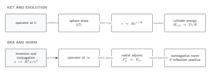
Plane–cylinder correspondence for the local vacuum sector. The Weyl factor converts a primary insertion to a cylinder operator, while $H_{\mathrm{cyl}}=D/R$ fixes excitation energies. Any additive vacuum energy and Lorentzian continuation require separate conventions. The diagram is schematic and not to scale.

Euclidean and Lorentzian cylinders

The metric above is Euclidean. Lorentzian cylinder time $t$ is obtained from a specified analytic continuation, for example $\tau=it$ together with the operator ordering and $i\epsilon$ prescription appropriate to the correlator. Euclidean decay $e^{-E\tau}$ then becomes Lorentzian phase evolution $e^{-iEt}$; the two should not be conflated before continuation.

Nor is the cylinder automatically thermal. A thermal trace requires periodic Euclidean time with period $\beta$, a choice of sectors and spin structure, and the density operator $e^{-\beta H}$. Radial quantization instead uses a noncompact logarithmic time coordinate. The thermal specialization is developed in Thermal States and One-Point Data.

The strongest general conclusion is therefore about relative spectra and separated-point correlators: conformal dimensions are cylinder excitation energies, and primary correlators transform by known Weyl factors. Absolute vacuum response, anomalies, contact terms, and thermal identifications require their own data.

References

• Rychkov, Slava. EPFL Lectures on Conformal Field Theory in $D\geq3$ Dimensions. SpringerBriefs in Physics. Cham: Springer, 2017. doi:10.1007/978-3-319-43626-5. Open PDF.
• Simmons-Duffin, David. “The Conformal Bootstrap.” In New Frontiers in Fields and Strings, 1–74. Singapore: World Scientific, 2017. doi:10.1142/9789813149441_0001. Open PDF.