

Large-N and Sparse-Spectrum CFT Data
A large-N CFT is not defined merely by a large numerical label. It is a family of theories with a controlled small parameter, a normalized set of operators, and a hierarchy of connected correlators. Spectral sparsity is a separate hypothesis. Together they organize crossing into single-trace input and multi-trace-like output, but neither hypothesis alone asserts a bulk dual.
Required background. Large-N CFT Data and Vector Models supplies concrete vector-model and generalized-free benchmarks. Large-N Factorization and Master-Field Claims supplies the underlying factorization expansion. Helpful background. Subleading Corrections, Double Scaling, and Nonuniform Limits explains why large-N and spectral limits need not commute.
Factorization as an intrinsic CFT statement
Section titled “Factorization as an intrinsic CFT statement”Choose unit-normalized primaries whose dimensions have finite limits as a parameter . A convenient factorization convention is
The choice of absorbs model-dependent powers of . For matrix-like examples one often has . In the unit-normalized vector-singlet benchmark on Large-N CFT Data and Vector Models, connected -point functions scale as , so the convention here is reproduced by . What matters for crossing is the measured hierarchy, not the name assigned to the parameter.
For an identical scalar with unit two-point function,
At leading order, factorization gives the generalized-free result
Its OPE contains towers customarily denoted ; their block decomposition is a standard solvable bootstrap benchmark Poland, Rychkov, and Vichi 2019, §6. Their leading dimensions are
and even for identical bosons. At order their dimensions and squared OPE coefficients become
This “double-trace” terminology describes the limiting factorized algebra. At finite , operator mixing can make the individual basis elements ambiguous; the dilatation eigenvalues and basis-invariant OPE combinations remain physical. The order-by-order structure follows from crossing and factorization, as developed in Heemskerk et al. 2009, §§2–4.
What sparse spectrum means
Section titled “What sparse spectrum means”Sparsity must identify a sector. A common large-gap condition selects a finite set of low-dimension single-trace primaries and defines
Then is a gap to additional higher-spin single-trace operators. This definition does not remove:
- the identity, stress tensor, and declared conserved currents;
- chosen low-dimension scalar or spinful primaries;
- the double-trace towers forced by factorization;
- possible dense sectors not covered by the declaration.
A scalar gap, a twist gap, and a higher-spin gap are inequivalent. So are “large compared with one,” “large compared with every light dimension,” and “taken to infinity after .” Every application must say which one it uses.
Classifying a four-point data set
Section titled “Classifying a four-point data set”Suppose the order- correlator contains one additional scalar of dimension and OPE coefficient . The crossed-channel exchange of creates logarithms such as
whose coefficients determine appropriate averages of . A crossing solution therefore has three logically distinct parts:
- declared single-trace data such as ;
- induced double-trace anomalous dimensions and OPE corrections;
- homogeneous crossing solutions, including contact-type terms, not fixed by the exchange poles alone.
Degeneracy matters. If several operators share the same leading dimension, a single correlator determines weighted averages such as
not every eigenvalue. Mixed correlators or additional symmetry data are required to resolve the matrix.
The inference boundary
Section titled “The inference boundary”The diagram below should be read from left to right. Solid arrows are CFT deductions once their labels are satisfied; the final dashed arrows are optional interpretations requiring a separate holographic dictionary.
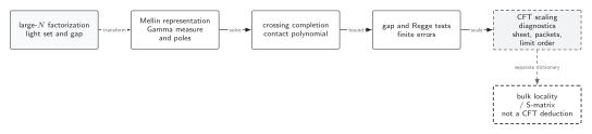
Large-N counting, spectral sparsity, Mellin analyticity, Regge boundedness, and uniform scaling limits are independent inputs. They support progressively stronger CFT-side conclusions; particles, local vertices, and an S-matrix remain optional later interpretations. The map is schematic.
The relationships encoded in the figure are:
| Input | Check performed in this chapter | CFT conclusion | Not established |
|---|---|---|---|
| connected-correlator hierarchy | normalization and power counting | factorized expansion and double-trace towers | a bulk Fock space |
| selected low primaries plus higher-spin gap | sector, spin, and limit order | sparse single-trace input | a finite bulk field content |
| Mellin poles and Gamma measure | contour, residues, and crossing | OPE exchange data | propagating bulk particles |
| bounded contact-polynomial basis | Regge degree and low-spin support | complete stated ambiguity | a local bulk vertex basis |
| gap-suppressed hierarchy | finite-gap remainder and uniformity | conditional low-energy CFT expansion | bulk locality |
| smeared Lorentzian or large-variable limit | sheet, normalization, convergence | controlled CFT scaling distribution | a physical S-matrix |
Order of limits and failure tests
Section titled “Order of limits and failure tests”Write the correlator as . The two limits
need not agree. Nor does a fixed- expansion control a Lorentzian configuration in which approaches a singular surface as a function of . A valid data classification therefore records:
- the operator normalization and exact definition of ;
- the expansion order and omitted remainder;
- the light-operator list and sector-specific gap;
- spin, symmetry, and degeneracy labels;
- the mixing quantities actually determined;
- every limit and its order;
- whether the claimed estimate is pointwise, averaged, or distributional.
The classification fails if changing the operator normalization changes the assigned power of without a corresponding convention update, if a dense double-trace tower is called a violation of single-trace sparsity, or if a large gap is inferred from checking only finitely many low spins.
Common pitfalls
Section titled “Common pitfalls”Calling every low-dimension operator single-trace. Single-trace is an asymptotic factorization class, not a dimension cutoff. Its definition requires a large-N operator basis and power counting.
Treating a gap as a complete spectrum. A higher-spin gap leaves declared low-spin operators and all multi-trace-like towers. State the sector and excluded exceptions.
Promoting factorization to locality. Factorization provides a perturbative algebraic organization. Polynomial boundedness, gap control, causality, and uniformity are additional tests Fitzpatrick and Kaplan 2013, §§2–4.
Exercises
Section titled “Exercises”Assume with unit normalized. Show why an additional primary exchanged at this order has , provided its conformal block is and no cancellation is imposed.
Solution
The conformal-block coefficient is . To contribute at order while the normalized block stays finite, and hence . The conclusion concerns the chosen unit normalization; rescaling changes both its two-point function and the quoted three-point coefficient.
References
Section titled “References”- Fitzpatrick, A. L., and Kaplan, J. “AdS Field Theory from Conformal Field Theory.” Journal of High Energy Physics 2013, 054 (2013). arXiv. DOI.
- Heemskerk, I., Penedones, J., Polchinski, J., and Sully, J. “Holography from Conformal Field Theory.” Journal of High Energy Physics 2009, 079 (2009). arXiv. DOI.
- Poland, D., Rychkov, S., and Vichi, A. “The Conformal Bootstrap: Theory, Numerical Techniques, and Applications.” Reviews of Modern Physics 91, 015002 (2019), §§5–6. arXiv. DOI.