Perturbative CFT Data near Free Fixed Points

A weakly coupled fixed point turns renormalized perturbation theory into CFT data: fixed-point anomalous dimensions become scaling dimensions, renormalized three-point functions become OPE coefficients, and equations of motion determine multiplet recombination. The conversion is reliable only after operator mixing, scheme dependence, evanescent structures, and the asymptotic character of the expansion have been controlled.

Required background. Free and generalized-free theories supplies the zeroth-order operator basis and Wick contractions. Beta functions, running masses, and field anomalous dimensions supplies the RG definitions. Helpful background. Operator mixing and renormalization matrices develops the matrix problem, and Gaussian and Wilson–Fisher fixed points gives the RG setting.

From renormalized operators to conformal eigenoperators

Let $g^I$ denote dimensionless renormalized couplings and let a finite set of operators with identical quantum numbers obey

$$\mathcal O_A^{\mathrm{bare}}=Z_A{}^B(g,\epsilon)\mathcal O_B(\mu), \qquad \gamma_A{}^B=(Z^{-1})_A{}^C\,\mu\frac{dZ_C{}^B}{d\mu}.$$

This sign convention makes the fixed-point dilatation matrix

$$D_A{}^B=\Delta_A^{(0)}\delta_A{}^B+\gamma_A{}^B(g_*), \qquad \beta^I(g_*)=0.$$

The scaling dimensions are its eigenvalues. When the zeroth-order dimensions are degenerate, diagonalizing only the diagonal entries of $\gamma$ is wrong: one must include every operator that mixes, including total derivatives and equation-of-motion operators, and then pass to conformal primaries or the appropriate quotient. In a unitary fixed point, the two-point matrix gives the inner product with respect to which the physical dilatation operator is self-adjoint; a nonsymmetric matrix in a convenient renormalization basis need not signal complex dimensions.

An OPE coefficient requires one more step. Renormalized two- and three-point functions contain normalization matrices and scheme-dependent finite pieces. Transform all operators to eigenoperators, normalize their separated-point two-point functions to the declared convention, and only then read the coefficient of the conformal three-point structure. This procedure makes fixed-point dimensions and normalized OPE coefficients invariant under analytic redefinitions of couplings and nonsingular changes of operator basis, order by order to the accuracy retained.

Wilson–Fisher data as a normalization test

Consider the Euclidean $O(N)$ model in $d=4-\epsilon$,

$$S=\int d^dx\left[ \frac12(\partial_\mu\phi_i)^2 +\frac{\mu^\epsilon g}{4!}(\phi_i\phi_i)^2 \right].$$

With this definition of $g$, minimal subtraction gives

$$\beta_g=-\epsilon g+\frac{N+8}{3}\frac{g^2}{16\pi^2}+O(g^3), \qquad g_*=\frac{48\pi^2}{N+8}\epsilon+O(\epsilon^2).$$

The first dimensions are

$$\begin{aligned} \Delta_\phi &=1-\frac\epsilon2 +\frac{N+2}{4(N+8)^2}\epsilon^2+O(\epsilon^3),\\ \Delta_{\phi^2,\,S} &=2-\frac{6}{N+8}\epsilon+O(\epsilon^2). \end{aligned}$$

The absence of an $O(\epsilon)$ anomalous part in $\Delta_\phi$ and the $O(\epsilon)$ shift of the singlet scalar are useful convention checks. The field equation

$$\partial^2\phi_i=\frac{\mu^\epsilon g}{6}\,\phi_i(\phi_j\phi_j)$$

also shows why the free primary $\phi_i(\phi_j\phi_j)$ becomes a descendant of $\phi_i$ at the interacting fixed point. This is conformal multiplet recombination, not the deletion of an operator. Its use in deriving Wilson–Fisher CFT data without evaluating every Feynman integral is explained in Rychkov and Tan 2015, §§1–4; the fixed-point expansion originates with Wilson and Fisher 1972, pp. 240–243.

Substituting $\epsilon=1$ into these first terms does not by itself produce a precision prediction for three dimensions. For example, at $N=1$ the displayed expressions give $\Delta_\phi\simeq0.5093$ and $\Delta_{\phi^2}\simeq1.333$, but omitted terms are not parametrically small at $\epsilon=1$. Resummation choices and independent bootstrap, Monte Carlo, or experimental comparisons are part of a quantitative conclusion.

What is universal at finite order

A coupling redefinition $g'^I=f^I(g)$ changes beta-function coefficients away from a fixed point and changes the coordinate value of $g_*$. At an isolated fixed point, however, the eigenvalues of

$$M^I{}_J=\left.\frac{\partial\beta^I}{\partial g^J}\right|_{g_*}$$

are invariant under a nonsingular reparameterization. So are properly normalized scaling dimensions and OPE coefficients. A truncated calculation preserves that invariance only up to the first omitted order: retaining a higher-order fixed-point root inside a lower-order anomalous dimension manufactures spurious precision.

Dimensional regularization introduces additional care for spinning and composite sectors. Tensor identities valid at an integer dimension do not hold in generic $d=4-\epsilon$, and evanescent operators can mix into physical operators through poles. The safe procedure is to work in a basis complete in generic $d$, renormalize, take the required quotient, and only then approach the target dimension. Degenerate operators require degenerate perturbation theory; near-degeneracies can make an apparently small off-diagonal term produce an order-one rotation of eigenvectors.

The schematic map below locates the Wilson–Fisher expansion among controlled higher-dimensional limits. Inspect the independent small parameter in each branch and the distinct way control can fail.

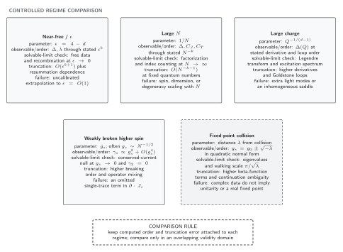
Controlled higher-dimensional CFT limits. The diagram is schematic and not to scale: proximity to a free point controls powers of $\epsilon$ or a weak coupling, whereas large $N$, large charge, and fixed-point collision use different expansions and different error tests.

The same information is available without the diagram:

Regime	Expansion parameter	Direct observable	Representative computed order	Error or remainder	Independent check	Leading loss of control
Near $d=4$ Wilson–Fisher	$\epsilon=4-d$	dimensions and OPE coefficients near the free basis	declared power of $\epsilon$ after fixed-point substitution	omitted powers and resummation dependence	multiplet recombination and an overlapping fixed-dimension method	evaluation at $\epsilon=O(1)$ without calibration
Weak gauge or Yukawa fixed point	loop-counting combinations of all $g_*^I$	mixed-operator spectrum and normalized correlators	declared loop order	omitted loops and competing roots	nonsingular scheme change	strong coupling or an unstable truncation
Large $N$	$1/N$	factorized spectrum and connected corrections	declared order in $1/N$	higher orders and nonuniform limits	index counting and crossing	spin or dimension scaling with $N$
Large charge	$Q^{-1/(d-1)}$	lowest dimension in a fixed-charge sector	declared derivative and Goldstone-loop order	higher derivatives and extra light modes	Legendre transform and excitation spectrum	a change of homogeneous ground state
Fixed-point collision	distance $\lambda$ from the collision	walking time and complex-conjugate data after continuation	local normal form through stated nonlinear order	higher beta-function terms and continuation ambiguity	scheme-invariant eigenvalues and multi-observable drift	mistaking slow real flow for a real fixed point

Error and failure tests

Fixed-point substitution. Check $\beta(g_*)$ to one order beyond the accuracy quoted where the available calculation permits. State which root is connected continuously to the free theory.

Scheme test. Perform an allowed finite redefinition and verify that fixed-point observables change only beyond the retained order. Couplings and individual matrix entries need not pass this test.

Mixing test. Enlarge the basis by redundant and evanescent operators, then verify that physical eigenvalues and normalized separated-point correlators are unchanged after the quotient.

Asymptotic test. Compare successive orders, vary admissible resummations, and test against an independent observable or method. A short asymptotic series supplies an estimate with assumptions, not a rigorous remainder bound.

A bounded calculation can be used for varying truncation order and comparing resummations once its executable implementation is available; no result on this page depends on that calculation having run.

Exercises

Using the displayed beta function, verify $g_*$ and compute the correction-to-scaling exponent $\omega=\beta_g'(g_*)$ through first order in $\epsilon$.

Solution

The nonzero root is $g_*=48\pi^2\epsilon/(N+8)+O(\epsilon^2)$. Differentiating gives $\beta_g'=-\epsilon+2(N+8)g/(48\pi^2)+O(g^2)$, hence $\omega=\epsilon+O(\epsilon^2)$.

Why must $g_*$ be substituted before diagonalizing the dilatation matrix?

Solution

Away from a fixed point, scale transformations also move the couplings, so the anomalous-dimension matrix alone is not the CFT dilatation operator. At $g_*$ the coupling flow vanishes and its eigenoperators have definite fixed-point scaling dimensions.

References

• Rychkov, S., and Tan, Z. M. (2015), “The $\epsilon$-expansion from conformal field theory,” Journal of Physics A: Mathematical and Theoretical 48, 29FT01. doi:10.1088/1751-8113/48/29/29FT01. Open PDF
• Wilson, K. G., and Fisher, M. E. (1972), “Critical exponents in 3.99 dimensions,” Physical Review Letters 28, 240–243. doi:10.1103/PhysRevLett.28.240