Nonunitary Sectors, Complex CFTs, and Fixed-Point Collisions

Fixed points can leave the real coupling space by collision, after which a real RG trajectory may run slowly between a complex-conjugate pair without ending at a real CFT. Complex conformal data can then organize an extended walking regime, but approximate power laws over a finite range are not evidence of an actual real fixed point. This page separates nonunitarity, reality, complex CFTs, and walking, and gives the local collision calculation with its scheme and evidence limits.

Required background. Fixed points and linearized RG flow supplies stability eigenvalues. Controlled interacting families supplies cross-method and extrapolation tests. Helpful background. Nonunitary and complex data in two-dimensional CFT gives exactly solvable examples and distinguishes negative norms from complex data.

Evidence cutoff. This research-sensitive synthesis includes sources and claims checked through 2026-08-09. Statements about particular candidate systems are conditional on the cited assumptions and should be reassessed when their continuum, spectral, or numerical evidence changes.

A local fixed-point collision

Let $t=\log\mu$ and adopt $\beta=dg/dt$. Near a generic collision controlled by a real parameter $\lambda$, an analytic shift and rescaling can put the one-dimensional center-manifold flow into the local form

$$\beta(g;\lambda)=(g-g_0)^2+\lambda$$

up to higher powers of $g-g_0$ and $\lambda$. This reduction assumes that one RG eigenvalue vanishes at the collision while all transverse directions can be solved as analytic functions of the center coordinate. If several eigenvalues vanish, a multi-coupling normal form is required.

For $\lambda<0$, there are two real fixed points,

$$g_\pm=g_0\pm\sqrt{-\lambda}, \qquad \beta'(g_\pm)=\pm2\sqrt{-\lambda}.$$

If $g$ couples to an operator $\mathcal O$ and the convention is $\Delta_\mathcal O=d+\beta'(g_*)$, then

$$\Delta_{\mathcal O,\pm}=d\pm2\sqrt{-\lambda}.$$

At $\lambda=0$ the fixed points coalesce and this operator is marginal to linear order. For $\lambda>0$, the roots and dimensions continue to

$$g_\pm=g_0\pm i\sqrt\lambda, \qquad \Delta_{\mathcal O,\pm}=d\pm2i\sqrt\lambda.$$

The square-root branching is invariant information about the local bifurcation. The exact polynomial form of $\beta$, the coordinate $g_0$, and higher coefficients are scheme-dependent. A nonsingular analytic redefinition maps the two roots and preserves the eigenvalues at each root; a singular transformation at the collision is not an admissible scheme comparison.

Walking and the exponential hierarchy

For real $g$ and $\lambda>0$, the beta function has no zero but is small near $g_0$. The RG time spent crossing a symmetric interval $g-g_0\in[-G,G]$ is

$$\Delta t =\int_{-G}^{G}\frac{dx}{x^2+\lambda} =\frac{2}{\sqrt\lambda} \arctan\!\left(\frac{G}{\sqrt\lambda}\right).$$

When $G\gg\sqrt\lambda$ while the local normal form remains valid,

$$\lvert\Delta t\rvert\simeq\frac{\pi}{\sqrt\lambda}, \qquad \frac{\mu_{\mathrm{UV}}}{\mu_{\mathrm{IR}}} \sim \exp\!\left(\frac{\pi}{\sqrt\lambda}\right).$$

The sign of $\Delta t$ depends on whether the trajectory is followed toward the UV or IR; the hierarchy uses its magnitude. Higher beta-function terms change the nonuniversal endpoints and prefactor but preserve the leading essential singularity when the simple collision normal form applies. This mechanism and its interpretation through complex CFT data are developed in Gorbenko, Rychkov, and Zan 2018, §§2.2 and 6.

Walking is approximate scale invariance over a finite interval. Effective dimensions can drift with scale, different observables can enter and leave the interval at different rates, and the ultimate infrared theory may be massive or a weak first-order transition. A large but finite correlation length is compatible with this picture; it is not by itself a real fixed point.

Nonunitary, real, and complex are different

Unitarity concerns the Hilbert-space inner product or Euclidean reflection positivity. Reality concerns whether the theory admits an antilinear involution that maps correlators to their complex conjugates. These conditions are logically distinct; the correlator-based distinction used here follows Gorbenko, Rychkov, and Zan 2018, §§6.1–6.2.

• A unitary CFT is real and has positive norms in the physical operator space.
• A real nonunitary CFT may have negative- or zero-norm states while retaining a reality involution. The Yang–Lee minimal model, with real $c=-22/5$, real dimensions, and a suitable reality convention for its correlators, is an example Gorbenko, Rychkov, and Zan 2018, §6.2.1.
• A real CFT with complex dimensions must contain conjugate operator data paired by the reality involution. Complex dimensions already exclude unitarity, but not reality.
• A complex CFT need not contain the conjugate of each datum internally. Its complex-conjugate CFT is a distinct partner. Dimensions, OPE coefficients, and central-charge analogues can be genuinely complex while conformal covariance, the OPE, and crossing remain meaningful.

An analytic continuation of a path integral must specify the integration cycle in complexified field space. Writing a complex coupling without a contour does not define a measure, and continuing a convergent real contour can cross Stokes walls. Correlators obtained on a chosen cycle need not satisfy reflection positivity. Similarly, a nonunitary subsector arising from ghosts, replicas, evanescent operators, or analytic continuation does not inherit positivity merely because a related parent construction has a unitary regime.

For the collision above, the two complex roots naturally describe conjugate complex CFTs. Perturbing their data can approximate real walking observables because conjugate imaginary parts can combine into real functions along the real trajectory. This does not turn either complex CFT into a physical endpoint of that real flow.

What finite data can establish

A numerical or experimental study over a finite size range can distinguish several levels of conclusion:

1. Slow flow: dimensionless observables vary weakly over an identified range. This is directly observable but does not choose a mechanism.
2. Collision-compatible drift: fitted effective exponents and the scale hierarchy follow a common collision normal form, with stable results under changes of fitting window and observable.
3. Complex-CFT organization: analytically continued dimensions and OPE data obey crossing and reproduce the walking corrections within a controlled expansion.
4. Real fixed point: infinite-volume or continuum evidence supports scale-independent real CFT data and rules out a finite correlation length. Walking evidence alone does not reach this conclusion.

Finite-size mimicry is especially dangerous when the walking length exceeds all simulated sizes. A stable-looking exponent can then be a local slope rather than a fixed-point dimension. Tests should include drift with size, the ultimate correlation length or latent discontinuity where accessible, alternative microscopic regulators, and observables not used in the fit.

The schematic diagram below places complex-fixed-point continuation beside other controlled higher-dimensional regimes. Inspect that this branch is explicitly nonunitary and carries its own expansion parameter and error tests.

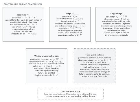
Controlled-regime comparison including a nonunitary complex-fixed-point continuation. The shared picture is schematic and not to scale; the collision law, conjugate roots, and walking hierarchy are derived separately on this page and summarized in the structured table below.

The collision panel has the following semantic description:

Parameter regime	Fixed points	Deformation dimension in the stated beta convention	Computed order	Error or independent check	Real-flow behavior and conclusion
$\lambda<0$	$g_0\pm\sqrt{-\lambda}$, both real	$d\pm2\sqrt{-\lambda}$	quadratic normal form	verify eigenvalues under a nonsingular scheme change; higher terms shift root coordinates	two real branches exist locally; flow direction follows the sign of $\beta'$
$\lambda=0$	double root at $g_0$	$d$ to linear order	first nonzero nonlinear beta term	include additional marginal directions if present	collision point; nonlinear terms decide the flow
$\lambda>0$	$g_0\pm i\sqrt\lambda$	$d\pm2i\sqrt\lambda$	quadratic normal form and leading small-$\lambda$ hierarchy	higher beta terms change endpoints; compare several observables	no real zero; a complex pair can organize walking time $\pi/\sqrt\lambda$
finite observation window	not determined solely by an apparent plateau	fitted effective dimension may drift	finite range in size or scale	vary range, regulator, and observable	approximate power laws cannot discriminate a real fixed point from walking without further limits

Failure tests and handoff

Scheme test. Repeat the local analysis after a nonsingular coupling redefinition. Root coordinates may move, but the collision type, conjugate pairing, and fixed-point eigenvalues must agree.

Reality test. State the antilinear involution or the path-integral cycle. Complex-conjugate numbers in a fit do not by themselves define a real theory.

Observable test. Extract the walking scale from several dimensionless observables and vary the fitting interval. Observable-dependent drift larger than the stated error weakens the one-coordinate normal form.

Thermodynamic test. Increase volume or correlation length until the proposed plateau is exited, or state that this limit remains unresolved. A finite accessible range cannot prove an infinite correlation length.

A bounded calculation can be used for integrating the normal form and testing synthetic finite-window fits once implemented. The evidence statements above do not presume an execution of that calculation.

Exercises

Evaluate the RG time from $g_0-G$ to $g_0+G$ and obtain its small-$\lambda$ limit.

Solution

Set $x=g-g_0$. The antiderivative is $\lambda^{-1/2}\arctan(x/\sqrt\lambda)$, so the interval gives $2\lambda^{-1/2}\arctan(G/\sqrt\lambda)$. For fixed $G>0$ and $\lambda\to0^+$, the arctangent approaches $\pi/2$, yielding $\pi/\sqrt\lambda$.

Show that the linearized RG eigenvalue is invariant under a nonsingular analytic redefinition $h=f(g)$.

Solution

$\beta_h=f'(g)\beta_g$. Differentiating with respect to $h$ and evaluating at a fixed point removes the term proportional to $\beta_g$, leaving $\partial_h\beta_h|_*=\partial_g\beta_g|_*$. This fails if $f'(g_*)=0$ or diverges, which is why singular maps are excluded.

References

• Gorbenko, V., Rychkov, S., and Zan, B. (2018), “Walking, weak first-order transitions, and complex CFTs,” Journal of High Energy Physics 2018(10), 108. doi:10.1007/JHEP10(2018)108. Open PDF