Mellin-Space CFT Correlators

Mellin space converts the multiplicative scaling structure of a conformal correlator into complex-variable analyticity. OPE families appear through pole sequences, spin appears through residue polynomials, and crossing acts by permuting Mellin variables. The Gamma-function measure is part of the representation: omitting it confuses universal double-trace poles with dynamical poles of the Mellin amplitude.

Required background. Conformal Partial Waves and the Shadow Formalism supplies spectral decompositions and projection contours. Mellin Transforms and Scaling Asymptotics supplies inversion and strip conditions. Helpful background. Dispersion Relations for CFT Correlators supplies the relation between growth and polynomial ambiguity.

Mellin variables and the Gamma measure

For scalar primaries of dimensions $\Delta_i$, a convention-independent starting point is

$$\left\langle\prod_{i=1}^n\mathcal O_i(x_i)\right\rangle =\int[d\delta]\,M(\delta_{ij}) \prod_{i<j}\Gamma(\delta_{ij})(x_{ij}^2)^{-\delta_{ij}},$$

subject to

$$\delta_{ij}=\delta_{ji}, \qquad \sum_{j\ne i}\delta_{ij}=\Delta_i.$$

Only $n(n-3)/2$ Mellin variables are independent. The integration lines are vertical and must separate the pole families appropriate to the chosen OPE domain. A formal expression without a nonempty fundamental strip, an analytic continuation prescription, or a distributional interpretation is not yet an inverse Mellin representation.

For four identical scalars of dimension $\Delta_\phi$, define

$$\delta_{12}=\delta_{34}=\Delta_\phi-\frac{s}{2}, \quad \delta_{14}=\delta_{23}=\Delta_\phi-\frac{t}{2}, \quad \delta_{13}=\delta_{24}=\Delta_\phi-\frac{u}{2},$$

with $s+t+u=4\Delta_\phi$. Factoring

$$\langle\phi_1\phi_2\phi_3\phi_4\rangle =\frac{\mathcal G(U,V)}{(x_{12}^2x_{34}^2)^{\Delta_\phi}},$$

gives the convention

$$\begin{aligned} \mathcal G(U,V) ={}&\int_{\mathcal C}\frac{ds\,dt}{(4\pi i)^2} U^{s/2}V^{t/2-\Delta_\phi} \Gamma^2\!\left(\Delta_\phi-\frac{s}{2}\right) \Gamma^2\!\left(\Delta_\phi-\frac{t}{2}\right)\\ &\times \Gamma^2\!\left(\Delta_\phi-\frac{u}{2}\right)M(s,t). \end{aligned}$$

For an initial Euclidean strip, the real parts can be chosen so that all three Gamma arguments are positive while their constrained sum is respected. Continuation beyond that strip requires moving contours and adding the residues of crossed poles. The power of $V$ and the definition of $u$ are convention choices; changing them requires transforming the entire measure, not just relabeling $M$.

OPE poles versus kinematic poles

The squared Gamma factors have poles at

$$s=2\Delta_\phi+2n, \qquad n=0,1,2,\ldots,$$

and in the crossed variables. These generate the generalized-free double-trace dimensions. They are present even when $M$ is a constant.

An exchanged primary $\mathcal O$ of dimension $\Delta$ and spin $J$ contributes a dynamical sequence

$$M(s,t)\supset \sum_{m=0}^{\infty} \frac{Q_{J,m}(t)}{s-(\Delta-J)-2m},$$

where $Q_{J,m}$ is a degree-$J$ Mack-type polynomial in the transverse Mellin variable, in a convention fixed by the conformal block normalization. Pole locations encode the primary twist and descendants; residues encode OPE coefficients and spin. This pole factorization is the central result of the Mellin representation Mack 2009, §§3–5 and Penedones 2011, §§2–3.

Three distinctions prevent common errors:

• a Gamma-measure pole is not an exchange pole of $M$;
• a finite list of principal poles is not a full conformal block unless its descendant sequence and residues are supplied;
• adding a crossing-symmetric polynomial changes the correlator but leaves the declared exchange-pole locations and residues unchanged.

Crossing and contact polynomials

For identical scalars, permutation symmetry acts on $(s,t,u)$ with $s+t+u=4\Delta_\phi$. In the present convention a fully symmetric correlator requires the correspondingly transformed Mellin integrand to agree. Its large-variable continuation must be matched to the chosen conformal Regge regime Costa, Gonçalves, and Penedones 2012, §§2–3. A contact-type solution has polynomial Mellin amplitude. The lowest examples are

$$M_0(s,t)=\lambda_0,$$

and

$$M_2(s,t)=\lambda_2\left(s^2+t^2+u^2\right),$$

up to lower-degree terms and convention-dependent shifts. Both are crossing symmetric. The degree controls large-variable growth and, after block decomposition, the range and asymptotics of affected double-trace data.

“Contact ambiguity” means ambiguity in reconstructing $M$ from specified pole or discontinuity data. Once the complete position-space correlator and transform convention are fixed, its Mellin amplitude is not freely ambiguous.

A declared contact-plus-pole toy

For algebraic checks, take

$$M_{\rm toy}(s,t) =\lambda_0+g_\chi^2 \left[ \frac{1}{s-\tau_\chi} +\frac{1}{t-\tau_\chi} +\frac{1}{u-\tau_\chi} \right].$$

It is symmetric under all permutations of $(s,t,u)$. Its three residues equal $g_\chi^2$, and shifting $\lambda_0$ changes no pole or residue. This is a deliberately truncated meromorphic fixture, not a conformal exchange amplitude: a physical scalar conformal block has the full descendant sequence $\tau_\chi+2m$ with fixed residues. The distinction makes the toy useful for testing pole extraction without overclaiming its spectrum.

A reproducible calculation should use a frozen constant-contact fixture and a separately declared exchange fixture. The equations above are the analytic baseline.

From data to a conditional inference

The figure summarizes which information survives each transformation. Inspect the contact branch: it rejoins the CFT correlator without passing through exchange-pole data.

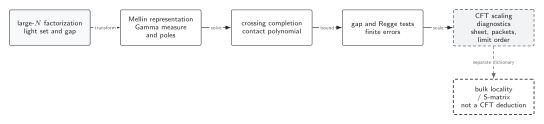
The Gamma measure, dynamical pole sequence, crossing-symmetric contact polynomial, Regge bound, and order of limits are separate parts of a Mellin analysis. Bulk terminology lies beyond the CFT-side inference boundary; the diagram is schematic.

Mellin object	How it is identified	Position-space content	Required qualification
Gamma measure	fixed by external dimensions and convention	generalized-free double-trace poles	contour and coincident-pole prescription
pole of $M$	residue of the meromorphic amplitude	exchanged primary twist and descendants	complete pole ladder and normalization
residue polynomial	degree and coefficients in transverse variable	spin and OPE data	Mack-polynomial convention
polynomial in $M$	entire crossing-symmetric addition	contact-type double-trace corrections	degree and Regge growth
large-$s,t$ scaling	asymptotics along a stated complex direction	Lorentzian or flat-space-type diagnostic	sheet, smearing, and uniform limit

Contour and normalization checks

A reliable calculation passes four independent tests:

1. Constraint: substituting the chosen $(s,t,u)$ reproduces every $\sum_{j\ne i}\delta_{ij}=\Delta_i$.
2. Crossing: all six point permutations map the complete integrand—including powers and Gamma factors—to the appropriate channel.
3. OPE closure: moving the $s$ contour in the declared direction gives the expected small-$U$ powers and logarithms.
4. Inverse transform: transforming back reproduces the correlator in an overlap domain, with tail and contour errors stated.

A residue calculation performed on $M$ alone does not test the inverse transform. Conversely, fitting the full integrand without dividing out the Gamma measure does not identify the dynamical poles.

Common pitfalls

Dropping Gamma factors. They are not a decorative normalization; they carry the universal double-trace structure. A pole classification without them is physically misidentified.

Calling every polynomial a harmless ambiguity. It is harmless only relative to the pole data used for reconstruction. It changes double-trace CFT data and may violate a declared Regge bound.

Taking a large real Mellin variable without a contour prescription. Mellin amplitudes are complex functions. The direction, fixed ratios, avoided poles, and analytic continuation all matter.

Exercises

Verify that $M_{\rm toy}$ is invariant under $s\leftrightarrow t$ and that adding $c(s^2+t^2+u^2)$ leaves all three simple-pole residues unchanged.

Solution

The three denominators are permuted by $s\leftrightarrow t$, while $u=4\Delta_\phi-s-t$ is unchanged. The degree-two addition is entire, so it contributes no coefficient to $(s-\tau_\chi)^{-1}$, $(t-\tau_\chi)^{-1}$, or $(u-\tau_\chi)^{-1}$. It therefore preserves the pole residues while changing the inverse Mellin transform.

References

• Costa, M. S., Gonçalves, V., and Penedones, J. “Conformal Regge Theory.” Journal of High Energy Physics 2012, 091 (2012). arXiv. DOI.
• Mack, G. “D-Dimensional Conformal Field Theories with Anomalous Dimensions as Dual Resonance Models.” Bulgarian Journal of Physics 36 (2009): 214–226. arXiv.
• Penedones, J. “Writing CFT Correlation Functions as AdS Scattering Amplitudes.” Journal of High Energy Physics 2011, 025 (2011). arXiv. DOI.