Thermal Inversion and Sum Rules

Thermal inversion extracts the coefficients of a local thermal OPE from a known two-point function. Euclidean angular orthogonality already identifies the data; a Lorentzian contour deformation rewrites the answer in terms of a discontinuity and reveals large-spin structure. That deformation is conditional: its analytic cuts, polynomial-growth exponent, arc terms, and integer-spin domain must be stated before residues are interpreted as thermal one-point data.

Required background. Thermal OPE and KMS crossing fixes the coefficient normalization and ordered correlator, while the Lorentzian inversion formula supplies the contour and spin-analyticity logic. Helpful background. Tauberian theorems and asymptotic spectral data clarifies why a large-spin or large-dimension reconstruction need not determine isolated low-lying data.

Literature cutoff. Statements about thermal inversion methods and applications reflect sources available through 2026-08-09. The general large-boost bound needed to eliminate arcs is treated as a hypothesis, not as an established theorem for every interacting CFT.

Euclidean partial waves and thermal data

Take the normalized two-point function of an identical bosonic scalar in the neutral canonical state on $S^1_\beta\times\mathbb R^{d-1}$. Set $\beta=1$ temporarily and use

$$G(\tau,\mathbf x) =\sum_{\mathcal O} a_{\mathcal O} C_J^{(\nu)}(\eta) r^{\Delta_{\mathcal O}-2\Delta_\phi}, \qquad \nu=\frac{d-2}{2},$$

with

$$a_{\mathcal O} =\frac{f_{\phi\phi\mathcal O}b_{\mathcal O}} {c_{\mathcal O}} \frac{J!}{2^J(\nu)_J}.$$

Complexify the trial dimension $\Delta$ and represent the OPE by

$$G(\tau,\mathbf x) =\sum_{J=0}^{\infty} \int_{\gamma_\Delta}\frac{d\Delta}{2\pi i} a(\Delta,J)C_J^{(\nu)}(\eta) r^{\Delta-2\Delta_\phi}.$$

Physical operators appear as simple poles,

$$a(\Delta,J) \sim-\frac{a_{\mathcal O}} {\Delta-\Delta_{\mathcal O}}.$$

The minus sign comes from closing the $\Delta$ contour clockwise to the right for $r<1$. A Euclidean inversion that has precisely these poles is

$$a_E(\Delta,J) =\frac1{N_J} \int_{r<r_0}d^dx\, C_J^{(\nu)}(\eta) r^{2\Delta_\phi-\Delta-d} G(\tau,\mathbf x), \qquad r_0<1,$$

where $N_J$ is fixed by Gegenbauer orthogonality on $S^{d-1}$. Taking $r_0<1$ keeps the integral strictly inside the OPE domain, so its $\Delta$ poles come only from the short-distance expansion. Restoring units sends $r_0<1$ to $r_0<\beta$ and restores the appropriate powers of $\beta$.

This formula is enough for a solvable extraction: expand a known correlator in angular harmonics, perform the radial Mellin integral, and read $a_{\mathcal O}$ from minus the residue. It does not by itself expose crossed-channel or large-spin information, which motivates the Lorentzian deformation Iliesiu et al. 2018, §§ 3.1–3.2.

The continuation and its cuts

Use spatial rotations to align $\mathbf x$ along one Euclidean coordinate $x_E$ and define

$$z=\tau+ix_E, \qquad \bar z=\tau-ix_E, \qquad z=rw, \qquad \bar z=rw^{-1}.$$

In Euclidean signature, $w$ lies on the unit circle. Continue the spatial coordinate as

$$x_E=-ix_L,$$

so $z,\bar z$ become independent real variables. The thermal coordinate $\tau$ remains Euclidean and periodic. This is not the usual real-time thermal continuation $\tau\to it$: $x_L$, not $\tau$, plays the Lorentzian time in the inversion kinematics.

At fixed $0<r<1$, the derivation assumes analyticity in the complex $w$ plane away from the cuts

$$(-\infty,-1/r), \quad (-r,0), \quad (0,r), \quad (1/r,\infty),$$

with the boundary value chosen consistently in the upper or lower half-plane. Use the discontinuity convention

$$\operatorname{Disc}G(z,\bar z) =\frac1i \left[G(z+i0,\bar z)-G(z-i0,\bar z)\right].$$

Changing this convention by a factor of two changes every recovered residue. The relevant large-boost limit is

$$w\to\infty, \qquad z\to\infty, \qquad \bar z\to0, \qquad z\bar z=r^2\text{ fixed},$$

and its $w\to0$ image. It follows a nearly lightlike trajectory around the thermal circle.

Discontinuity, arcs, and the spin threshold

Assume the continued correlator obeys the polynomial bound

$$G(rw,rw^{-1})=O(\lvert w\rvert^{J_0})$$

uniformly in the half-plane used to deform the contour, with the corresponding $w\to0$ bound. For integer spin $J>J_0$, the large and small arcs vanish. In $d>2$, the result can be written

$$\begin{aligned} a(\Delta,J) &=a_{\mathrm{disc}}(\Delta,J) +\theta(J_0-J)a_{\mathrm{arc}}(\Delta,J),\\ a_{\mathrm{disc}}(\Delta,J) &=(1+(-1)^J)K_J \int_0^1\frac{dz}{z} \int_1^{1/z}\frac{d\bar z}{\bar z} \,\mathcal K_{\Delta,J}(z,\bar z) \operatorname{Disc}G(z,\bar z),\\ K_J&=\frac{\Gamma(J+1)\Gamma(\nu)} {4\pi\Gamma(J+\nu)}. \end{aligned}$$

The explicit kernel $\mathcal K_{\Delta,J}$ combines the radial powers, the angular measure with its prescribed branch, and the solution of the Gegenbauer equation that decays on the deformed contour; the complete convention is Iliesiu et al. 2018, eqs. (3.14)–(3.17). Writing the domain and normalization while leaving the kernel named is safer than mixing kernels from different discontinuity or Gegenbauer conventions.

The factor $1+(-1)^J$ projects the identical-scalar problem onto even integer spin. Analytic continuation in $J$ is possible only after fixing the branch of the kernel and establishing the growth bound. The output has poles in $\Delta$ whose residues give $-a_{\mathcal O}$ in the normalization above.

For $J\le J_0$, the discontinuity is incomplete:

$$a(\Delta,J) =a_{\mathrm{disc}}(\Delta,J) +a_{\mathrm{arc}}(\Delta,J).$$

The arc term is the thermal analogue of a subtraction contribution. It depends on the large-$w$ behavior of the full correlator and can cancel apparent low-spin poles from the discontinuity integral. Local contact terms and polynomial pieces can have zero discontinuity and reside entirely in this subtraction data. Therefore a discontinuity-only scalar answer is not justified merely because the integral converges numerically.

The foundational derivation explicitly notes that no general rigorous upper bound on $J_0$ was established for $d>2$ Iliesiu et al. 2018, § 3.5, pp. 22–24. In a model, determine or bound $J_0$ from the complete correlator; do not infer it term by term in a perturbative expansion whose large-boost limit may be nonuniform.

A mean-field residue check

For the generalized-free image correlator,

$$G(\tau,\mathbf x) =\sum_{m\in\mathbb Z} \frac1{[(\tau+m)^2+\lvert\mathbf x\rvert^2]^{\Delta_\phi}},$$

the thermal OPE contains the identity and double-twist operators $[\phi\phi]_{n,J}$ with

$$\Delta_{n,J}=2\Delta_\phi+2n+J, \qquad J\in2\mathbb Z_{\ge0}.$$

Direct expansion gives

$$a_{[\phi\phi]_{n,J}} =2\zeta(2\Delta_\phi+2n+J) \frac{(J+\nu)(\Delta_\phi)_{J+n} (\Delta_\phi-\nu)_n} {n!(\nu)_{J+n+1}}.$$

The poles of the inversion integral reproduce these coefficients Iliesiu et al. 2018, § 4, eqs. (4.6)–(4.14). In the free scalar case $\Delta_\phi=\nu$, only $n=0$ survives and the conserved even-spin currents obey

$$a_{J}=2\zeta(d-2+J).$$

For example, the spin-two coefficient is $2\zeta(d)$ in this thermal-block normalization. This is a check of the product $f_{\phi\phi J}b_J/c_J$ with the stated Gegenbauer factor, not a convention-independent value of $b_J$ alone.

At $d=3,J=0$, the expression contains $\zeta(1)$ and diverges: the free scalar zero mode invalidates the naive thermal fixture. For low spin in interacting examples, arc contributions can likewise be essential. A successful high-spin match does not license extrapolation through those exceptions.

KMS sum rules as an independent extraction

In the common OPE domain, identical-boson KMS symmetry gives

$$\left. \partial_\tau^{2m+1}G(\tau,\mathbf x) \right|_{\tau=1/2}=0.$$

Substitution of the thermal blocks yields

$$\sum_{\mathcal O} a_{\mathcal O} \left. \partial_\tau^{2m+1} \left[ C_J^{(\nu)}(\eta) r^{\Delta_{\mathcal O}-2\Delta_\phi} \right] \right|_{\tau=1/2} =0.$$

These equations require no Lorentzian contour, but they also have no general coefficient positivity. They are useful checks on inversion: residues reconstructed from a correlator should satisfy the KMS derivatives within a separately bounded OPE tail.

Let $G=G_{\le\Lambda}+R_\Lambda$ in a compact subset of the OPE overlap. If

$$\left\lvert \partial_\tau^{2m+1}R_\Lambda \right\rvert \le\varepsilon_{m,\Lambda},$$

then the truncated KMS sum must vanish within $\varepsilon_{m,\Lambda}$. For the Lorentzian integral, an error envelope $\lvert\delta G\rvert\le\varepsilon(z,\bar z)$ gives

$$\lvert\delta a_{\mathrm{disc}}\rvert \le(1+(-1)^J)K_J \int_0^1\frac{dz}{z} \int_1^{1/z}\frac{d\bar z}{\bar z} \left\lvert\mathcal K_{\Delta,J}\right\rvert \varepsilon(z,\bar z),$$

when the weighted integral converges. Endpoint amplification by the kernel is why a uniform Euclidean residual alone need not control inversion.

The inversion flow and its structured equivalent

The diagram shows where exact data stop and hypothesis-dependent steps begin. Inspect the branch at the large-boost contour: it either vanishes for $J>J_0$ or supplies an arc term.

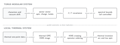
A normalized scalar thermal correlator first defines Euclidean OPE poles. Analytic continuation in a spatial direction produces Lorentzian cuts; a discontinuity integral recovers even-spin data only with the declared analyticity and polynomial-growth hypotheses. Arc or subtraction terms retain low-spin and contact information. The torus modular branch in the same schematic remains a distinct global constraint.

The complete logic is also recorded in the table:

Step	Input and domain	Output	Required hypothesis	Term not fixed by the step
Euclidean inversion	normalized $G$ on $r<r_0<\beta$	poles in $\Delta$ with residues $-a_{\mathcal O}$	OPE convergence and Gegenbauer normalization	changes analytic in $\Delta$ away from physical poles
Spatial Lorentzian continuation	$x_E=-ix_L$ at fixed Euclidean $\tau$	independent real $z,\bar z$ and specified cuts	chosen boundary value and no extra singularities crossed	ordinary real-time thermal ordering is not produced
Contour deformation	fixed $r$, complex $w$	discontinuity integral	analyticity off the declared cuts	arcs at zero and infinity
High-spin inversion	integer even $J>J_0$	$a_{\mathrm{disc}}(\Delta,J)$	uniform $O(\lvert w\rvert^{J_0})$ growth bound	none from the arc if the bound is proved
Low-spin inversion	$J\le J_0$	$a_{\mathrm{disc}}+a_{\mathrm{arc}}$	explicit large-boost or subtraction data	contact, polynomial, and other zero-discontinuity terms
Truncated reconstruction	finite images, spectrum, or integration grid	approximate residues and KMS moments	weighted tail and quadrature bounds varied independently	unbounded endpoint or low-spin error if those estimates fail

Recent applications continue to use thermal inversion for asymptotic heavy-state data in particular models; for example, a 2026 analysis treats a three-dimensional CFT associated with interacting scalar QFT in $AdS_4$ at fixed spin Burić et al. 2026, abstract. Such model-specific success does not replace the correlator-by-correlator arc and growth analysis above.

Common failure modes

Continuing the wrong coordinate. The inversion kinematics rotates a spatial coordinate while leaving $\tau$ Euclidean. Rotating $\tau$ produces different thermal real-time correlators and cuts.

Using a discontinuity-only formula at low spin. If $J\le J_0$, arc terms can carry or cancel physical poles. The scalar sector is especially sensitive.

Inferring a growth exponent term by term. Perturbative contributions can grow faster at successive orders even when the resummed correlator is bounded. Establish the bound for the object actually inverted.

Reading $b_{\mathcal O}$ without undoing normalization. The residue gives $a_{\mathcal O}$; recovering $b_{\mathcal O}$ requires $f_{\phi\phi\mathcal O}$, $c_{\mathcal O}$, and the Gegenbauer factor in the declared tensor convention.

Exercises

Suppose Euclidean inversion gives

$$a(\Delta,J)=-\frac{3}{\Delta-7}+\text{regular}.$$

What thermal OPE data does this encode?

Solution

There is a spin-$J$ operator of dimension $7$ with thermal-block coefficient $a_{\mathcal O}=3$, because the convention is $a(\Delta,J)\sim-a_{\mathcal O}/(\Delta-\Delta_{\mathcal O})$. The value of $b_{\mathcal O}$ follows only after dividing by $f_{\phi\phi\mathcal O}/c_{\mathcal O}$ and the stated spin-normalization factor.

Assume $G(rw,rw^{-1})=O(\lvert w\rvert^{1.4})$ uniformly on the relevant half-plane. For which nonnegative integer spins may the arc be dropped from the stated bound alone?

Solution

The contour argument requires $J>J_0=1.4$. Thus it removes the arc for integer $J\ge2$. In the identical-scalar sector only even spins occur, so the first applicable spin is $J=2$. Nothing in this assumption fixes $J=0$; its arc must be retained.

End of the thermal route

The robust workflow is: normalize the state and operators; establish the Euclidean OPE and KMS domain; bound image or spectral tails; choose the spatial Lorentzian boundary value; declare the discontinuity convention and large-boost exponent; retain arcs at low spin; and finally compare inversion residues with KMS sum rules. Each step has an independent failure mode, so agreement between the two extractions is a substantive check.

References

• Burić, Ilija, Francesco Mangialardi, Francesco Russo, Volker Schomerus, and Alessandro Vichi. “Thermal One-point Functions and Asymptotic CFT Data: QFT in AdS.” arXiv:2606.17167 [hep-th], 2026. Open preprint.
• Iliesiu, Luca, Murat Koloğlu, Raghu Mahajan, Eric Perlmutter, and David Simmons-Duffin. “The Conformal Bootstrap at Finite Temperature.” Journal of High Energy Physics 2018, no. 10 (2018): 070. doi:10.1007/JHEP10(2018)070. Open preprint.