Beta Functions, Running Masses, and Field Anomalous Dimensions

Beta functions and anomalous dimensions are the components of fixed-bare scale flow in a chosen set of renormalized coordinates. They are not read from an isolated counterterm by pattern matching: one first declares the bare–renormalized relations, includes the canonical $\epsilon$ terms of every coupling, and differentiates while all bare data are held fixed. In a minimal-subtraction scheme the result is determined by simple-pole residues, while the higher poles provide consistency checks.

This page derives that extraction rule for dimensionless couplings, masses, and fields. A one-loop real-scalar/Dirac-fermion Yukawa model then supplies a closed benchmark with a running Yukawa coupling, quartic coupling, scalar mass, and two field anomalous dimensions. The benchmark also shows how a formal Landau singularity or a negative running quartic marks the boundary of a perturbative trajectory rather than a trustworthy ultraviolet prediction.

Required background. Scale Independence and the Callan–Symanzik Equation defines fixed-bare differentiation and the field-sign convention. Dimensional Regularization and Minimal Subtraction supplies the $d=4-2\epsilon$ pole convention.

Helpful background. The 1PI Effective Action and Mean-Field Equations is useful for identifying which two- and three-point pole fixes each renormalization factor.

RG functions as fixed-bare velocities

For renormalized coordinates $g^i$, dimensionful parameters $a^A$, and fields $\Phi_r$, define

$$\begin{aligned} \beta^i &\equiv \mu\frac{dg^i}{d\mu}\bigg\rvert_0, \\ \beta_{a^A} &\equiv \mu\frac{da^A}{d\mu}\bigg\rvert_0, \\ \gamma_r &\equiv \frac12\mu\frac{d\ln Z_r}{d\mu}\bigg\rvert_0, \qquad \Phi_{0r}=Z_r^{1/2}\Phi_r . \end{aligned}$$

The field coordinate therefore evolves as

$$\mu\frac{d\Phi_r}{d\mu}\bigg\rvert_0 =-\gamma_r\Phi_r.$$

The final minus sign agrees with the 1PI equation on the preceding page. A source that defines $\mu\,d\Phi_r/d\mu=+\widetilde\gamma_r\Phi_r$ uses $\widetilde\gamma_r=-\gamma_r$.

For a mass squared it is clearest to keep the beta function itself:

$$\eta_{m^2} \equiv \frac{\beta_{m^2}}{m^2} = \mu\frac{d\ln m^2}{d\mu}\bigg\rvert_0.$$

The Callan–Symanzik convention used on the preceding page was

$$\gamma_{m^2}^{\rm CS} \equiv -\mu\frac{d\ln m^2}{d\mu}\bigg\rvert_0,$$

so $\gamma_{m^2}^{\rm CS}=-\eta_{m^2}$. Writing the translation once prevents a hidden sign change in the mass term of the RG operator.

Dimensionful and dimensionless coordinates

Suppose $a$ has engineering mass dimension $d_a$ in four dimensions. The associated dimensionless coordinate is

$$\widehat a(\mu)=\mu^{-d_a}a(\mu),$$

and its beta function is

$$\beta_{\widehat a} = \mu\frac{d\widehat a}{d\mu} = -d_a\widehat a +\mu^{-d_a}\beta_a.$$

Fixed points are zeros of beta functions for dimensionless coordinates. A nonzero constant mass is not a fixed point merely because $\beta_{m^2}=0$: for $\widehat m^2=m^2/\mu^2$,

$$\beta_{\widehat m^2} = \left(-2+\eta_{m^2}\right)\widehat m^2.$$

Near the Gaussian fixed point the $-2$ term makes the mass deformation relevant toward the infrared. This canonical term is logically separate from the loop-induced mass running.

Minimal-subtraction pole extraction

Let every marginal coupling have a declared continuation

$$g_0^i = \mu^{\kappa_i\epsilon} \left[ g^i +\sum_{n=1}^{\infty} \frac{a_n^i(g)}{\epsilon^n} \right],$$

where $\kappa_i$ records its engineering dimension in $d=4-2\epsilon$. A Yukawa coupling has $\kappa_y=1$, while a scalar quartic has $\kappa_\lambda=2$. Its $d$-dimensional beta function begins as

$$\beta_d^i = -\kappa_i\epsilon g^i+\beta^i(g).$$

Differentiate $g_0^i$ at fixed bare data:

$$0 = \kappa_i\epsilon g_0^i +\beta_d^j \frac{\partial g_0^i}{\partial g^j}.$$

The finite part comes from the explicit $\epsilon$ term multiplying the simple pole. Pole cancellation then gives

$$\boxed{ \beta^i(g) = \left( \sum_j\kappa_jg^j\frac{\partial}{\partial g^j} -\kappa_i \right) a_1^i(g). }$$

The higher poles do not supply independent RG functions. Their residues must satisfy recursive relations that cancel every remaining $1/\epsilon^n$ term. An uncancelled pole signals inconsistent lower-order counterterms or an incomplete parameter set. This simple-pole structure was established in the dimensional-renormalization analysis of ’t Hooft 1973, pp. 455–468 and is derived in the fixed-bare language in Collins 1984/2023, § 7.3.1, pp. 180–183.

For a multiplicatively renormalized mass parameter,

$$m_0^2 = m^2+\frac{b_1(g,m^2)}{\epsilon} +\text{higher poles},$$

the one-loop finite term is

$$\beta_{m^2} = \sum_j \kappa_jg^j \frac{\partial b_1}{\partial g^j}.$$

If several masses or relevant couplings share the same quantum numbers, $b_1$ is a linear combination of all of them and the mass beta function is a matrix equation. Additive heavy-mass terms cannot be represented by one number called a mass anomalous dimension.

For a field, write the square-root factor rather than $Z_r$ itself:

$$Z_r^{1/2} = 1+\frac{c_{r1}(g)}{\epsilon} +\text{higher poles}.$$

Then

$$\boxed{ \gamma_r = -\sum_j \kappa_jg^j \frac{\partial c_{r1}}{\partial g^j}. }$$

Using the pole of $Z_r$ instead of $Z_r^{1/2}$ without changing the prefactor creates the common factor-of-two error. In a mass-dependent subtraction scheme, explicit derivatives with respect to $m/\mu$ or external subtraction ratios must be included; the pure-pole formulas above are then insufficient.

A one-loop scalar–Yukawa benchmark

Consider one real scalar and one massless Dirac fermion with

$$\mathcal L = \frac12(\partial_\mu\phi)(\partial^\mu\phi) -\frac12m^2\phi^2 -\frac{\lambda}{4!}\phi^4 +\bar\psi\,i\gamma^\mu\partial_\mu\psi -y\phi\bar\psi\psi .$$

The discrete chiral transformation

$$\phi\mapsto-\phi, \qquad \psi\mapsto\gamma_5\psi, \qquad \bar\psi\mapsto-\bar\psi\gamma_5$$

forbids a fermion mass and odd powers of $\phi$. Thus the displayed parameter set closes at one loop. The normalization is one Dirac flavor, $\lambda\phi^4/4!$, and modified minimal subtraction in $d=4-2\epsilon$.

After translating the published $n=4+\epsilon$ convention to this page’s $d=4-2\epsilon$ convention, the one-loop bare relations are

$$\begin{aligned} y_0 &= \mu^\epsilon \left[ y+\frac{5y^3}{32\pi^2\epsilon} \right], \\ \lambda_0 &= \mu^{2\epsilon} \left[ \lambda +\frac{ 3\lambda^2+8\lambda y^2-48y^4 }{32\pi^2\epsilon} \right], \\ m_0^2 &= m^2 \left[ 1+\frac{\lambda+4y^2}{32\pi^2\epsilon} \right], \\ Z_\phi^{1/2} &= 1-\frac{y^2}{16\pi^2\epsilon}, \\ Z_\psi^{1/2} &= 1-\frac{y^2}{64\pi^2\epsilon}. \end{aligned}$$

These pole coefficients follow from the complete one-loop counterterms in Toms 2018, §§ 5.1–5.2, pp. 14–18.

Applying the weighted Euler operator gives

$$\begin{aligned} \beta_y &= \frac{5y^3}{16\pi^2}, \\ \beta_\lambda &= \frac{ 3\lambda^2+8\lambda y^2-48y^4 }{16\pi^2}, \\ \beta_{m^2} &= \frac{\lambda+4y^2}{16\pi^2}m^2, \\ \gamma_\phi &= \frac{y^2}{8\pi^2}, \\ \gamma_\psi &= \frac{y^2}{32\pi^2}. \end{aligned}$$

For example,

$$\begin{aligned} \beta_y &= \left( y\partial_y+2\lambda\partial_\lambda-1 \right) \frac{5y^3}{32\pi^2} = \frac{5y^3}{16\pi^2}, \\ \gamma_\phi &= -\left( y\partial_y+2\lambda\partial_\lambda \right) \left( -\frac{y^2}{16\pi^2} \right) = \frac{y^2}{8\pi^2}. \end{aligned}$$

The full extraction record is:

Quantity	Simple-pole input	One-loop RG function	Immediate check
Yukawa coupling $y$	$a_{y1}=5y^3/(32\pi^2)$	$\beta_y=5y^3/(16\pi^2)$	Cubic in $y$ and odd under $y\mapsto-y$
Quartic coupling $\lambda$	$a_{\lambda1}=(3\lambda^2+8\lambda y^2-48y^4)/(32\pi^2)$	$\beta_\lambda=2a_{\lambda1}$	Reduces to $3\lambda^2/(16\pi^2)$ at $y=0$
Scalar mass $m^2$	$b_1=m^2(\lambda+4y^2)/(32\pi^2)$	$\beta_{m^2}=m^2(\lambda+4y^2)/(16\pi^2)$	Multiplicative only because the fermion is massless and the symmetry closes the sector
Scalar field $\phi$	$c_{\phi1}=-y^2/(16\pi^2)$	$\gamma_\phi=y^2/(8\pi^2)$	Vanishes in the pure $\phi^4$ theory at one loop
Fermion field $\psi$	$c_{\psi1}=-y^2/(64\pi^2)$	$\gamma_\psi=y^2/(32\pi^2)$	One quarter of $\gamma_\phi$ in this one-flavor normalization

Every entry has the correct loop order and respects the discrete symmetry. Setting $y=0$ reproduces the scalar benchmark from the previous chapter; setting $\lambda=0$ does not define a closed trajectory because $\beta_\lambda=-3y^4/\pi^2$ remains nonzero.

Running, fixed rays, and stopping rules

Let

$$t=\ln\frac{\mu}{\mu_0}, \qquad Y\equiv y^2, \qquad Y_0=y^2(\mu_0).$$

The one-loop Yukawa equation is autonomous:

$$\frac{dY}{dt} = \frac{5}{8\pi^2}Y^2.$$

Its solution is

$$\boxed{ Y(\mu) = \frac{Y_0}{ 1-\dfrac{5Y_0}{8\pi^2} \ln(\mu/\mu_0) }. }$$

Thus $Y$ decreases toward the infrared and grows toward the ultraviolet. The formal one-loop singularity is

$$\mu_{\rm L} = \mu_0 \exp\left( \frac{8\pi^2}{5Y_0} \right).$$

Perturbation theory fails before the denominator literally vanishes, so $\mu_{\rm L}$ is a stopping estimate for this truncated trajectory, not evidence that the exact theory contains a physical pole.

The quartic flow is coupled to $Y$. The ratio

$$r\equiv\frac{\lambda}{Y}$$

obeys

$$\frac{dr}{d\ln Y} = \frac{3r^2-2r-48}{10}.$$

There are two fixed rays,

$$r_\pm = \frac{1\pm\sqrt{145}}{3}.$$

Only $r_+>0$ is compatible with a positive classical quartic. Along this ray,

$$\lambda(\mu)=r_+Y(\mu),$$

and the mass equation integrates to

$$\frac{m^2(\mu)}{m^2(\mu_0)} = \left[ \frac{Y(\mu)}{Y_0} \right]^{(r_++4)/10}.$$

For a generic positive initial quartic, the exact one-loop solution shows two regimes. If

$$\frac{\lambda_0}{Y_0} < \frac{1+\sqrt{145}}{3},$$

then $\lambda$ crosses zero before the formal Yukawa Landau singularity; above that ratio it grows. Toms gives the closed coupled solution and the crossing scale in Toms 2018, Appendix A, pp. 24–25. A zero crossing reached while all couplings remain perturbative is a warning that the assumed scalar potential is no longer stable in that range. Vacuum stability still requires an effective-potential analysis and any additional degrees of freedom present in the actual theory.

For the short-interval checks, write $m_{\rm ref}^2\equiv m^2(\mu_0)$. Evaluating the right-hand sides at $\mu_0$ gives

$$\begin{aligned} m^2(\mu) &= m_{\rm ref}^2 \left[ 1+ \frac{\lambda_0+4Y_0}{16\pi^2} \ln\frac{\mu}{\mu_0} \right] +\text{higher RG orders}, \\ \phi(\mu) &= \phi(\mu_0) \left[ 1-\frac{Y_0}{8\pi^2} \ln\frac{\mu}{\mu_0} \right] +\text{higher RG orders}, \\ \psi(\mu) &= \psi(\mu_0) \left[ 1-\frac{Y_0}{32\pi^2} \ln\frac{\mu}{\mu_0} \right] +\text{higher RG orders}. \end{aligned}$$

The field lines describe changes of renormalized coordinates. They become physical only after the external fields or operators are assembled into a properly normalized observable.

The characteristic diagram now has concrete inputs. Inspect panels (a) and (b): the pole residues above determine the vector field and the transport factors. Panel (c) deliberately shows the opposite, asymptotically free sign $\beta=-b_0g^3$; it is a comparison case, not the positive-beta Yukawa trajectory.

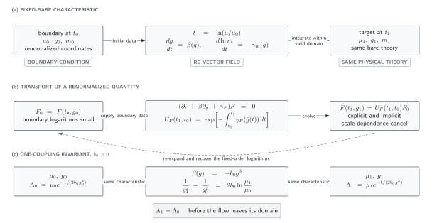
RG functions turn fixed-bare scale independence into characteristic flow. For the scalar–Yukawa benchmark, panels (a) and (b) use $\beta_y$, $\beta_\lambda$, $\beta_{m^2}$, $\gamma_\phi$, and $\gamma_\psi$ extracted above. Panel (c) is the distinct one-coupling case $\beta=-b_0g^3$ with $b_0>0$, for which $\Lambda=\mu e^{-1/(2b_0g^2)}$ is invariant within the truncated flow’s domain. The original diagram is schematic and not to scale.

Figure component	Scalar–Yukawa input or comparison	Verification
Fixed-bare vector field	$dY/dt=5Y^2/(8\pi^2)$ and $d\lambda/dt=(3\lambda^2+8\lambda Y-48Y^2)/(16\pi^2)$	Substitution into the bare pole relations gives zero through one loop
Mass transport	$d\ln m^2/dt=(\lambda+4Y)/(16\pi^2)$	On $r=r_+$, differentiation of the power solution returns the mass beta function
Field transport	$d\ln\phi/dt=-Y/(8\pi^2)$ and $d\ln\psi/dt=-Y/(32\pi^2)$	Re-expansion reproduces the one-loop field logarithms
Asymptotically free comparison	$\beta=-b_0g^3$, not $\beta_y>0$	Direct differentiation gives $d\ln\Lambda/d\ln\mu=0$

Scheme-dependent coordinates and invariant claims

Under a nonsingular finite change of coupling coordinates,

$$g'^i=f^i(g),$$

the beta function transforms as a vector field:

$$\beta'^i(g') = \frac{\partial f^i}{\partial g^j}\beta^j(g).$$

Under a finite field rescaling $\Phi'_r=C_r(g)\Phi_r$,

$$\gamma'_r = \gamma_r -\beta^i\partial_i\ln C_r.$$

These formulas separate coordinate data from invariant statements. The following table is the chapter’s reusable claims record:

Item	What may change	What survives a consistent translation	Required qualification or check
Renormalized $g^i$, masses, and field normalizations	Numerical values under finite scheme or basis changes	A prediction expressed in the same physical inputs	Translate every parameter and field factor through the retained order
Beta function away from a fixed point	Components and higher-order coefficients	The integral curves as geometric trajectories under a nonsingular coordinate map	Compare transformed vector fields, not coefficients at equal numerical coupling
Elementary-field anomalous dimension	Finite field rescaling; gauge parameter in a gauge theory	Scaling of a gauge-invariant observable after all factors are combined	Never identify a gauge-dependent elementary-field exponent with an observable
Exact fixed point	Coordinate location $g_\star^i$	Existence of the zero under a regular map	Exclude singular redefinitions and verify the fixed point lies in the method’s domain
Fixed-point stability data	Matrix representation and basis	Eigenvalues in a closed physical sector	Include operator mixing and redundant directions before diagonalizing
Transmuted scale	Its conventional normalization	Matched dimensionless ratios or predictions	State the scheme and reference condition defining the scale
Zero or singularity of a truncated beta function	Location and even apparent existence at insufficient order	Only the demonstrated breakdown of the stated approximation	Vary scheme/order and stop before couplings become large
Wilson coefficient versus power correction	Factorization scheme and, for an asymptotic series, summation prescription	Their consistently defined sum in an observable	Match the ambiguity of the perturbative term to the operator matrix element; developed on the renormalon page
Residual $\mu$ or scheme dependence	Numerical size at finite order	Vanishing in the exact consistently matched prediction	Treat the residual as a diagnostic, not a universal probability law

Finite renormalization prescriptions are coordinate changes of the type summarized here Collins 1984/2023, § 7.1, pp. 169–176. The power-correction row anticipates a later limitation: in dimensional factorization, a renormalon-ambiguous coefficient and the corresponding operator matrix element are separately prescription dependent, while their sum is unique Beneke 1999, § 2.3, pp. 14–17.

Gauge-parameter caution

The scalar–Yukawa benchmark has no gauge fixing, so its field anomalous dimensions are unambiguous within the declared subtraction convention. In a gauge theory, $Z_\psi$, $Z_A$, and their anomalous dimensions can depend on the gauge parameter. Off-shell Green functions inherit that dependence, while a physical observable must lose it after vertices, external residues, operator factors, and parameter translations are combined. Collins develops this cancellation and the status of gauge-dependent off-shell quantities in Collins 1984/2023, § 12.4, pp. 309–314.

Operator anomalous dimensions are matrices rather than elementary-field numbers. Their basis direction, transposition, and ordered evolution belong to Operator Anomalous-Dimension Matrices.

Common pitfalls

Dropping the canonical $\epsilon$ term. The finite beta function comes from $-\kappa_i\epsilon g^i$ multiplying a simple pole. Setting $\epsilon=0$ before differentiating loses precisely the term one is trying to compute.

Using the pole of the wrong renormalization factor. If the bare field is written with $Z^{1/2}$, use the simple pole of $Z^{1/2}$. Switching silently to the pole of $Z$ doubles the anomalous dimension.

Calling every mass beta function a mass anomalous dimension. A multiplicative mass permits $\beta_{m^2}/m^2$. Additive mixing with other masses or relevant parameters requires a vector or matrix and cannot be compressed into one logarithmic derivative.

Looking for fixed points in dimensionful parameters. Divide by the appropriate power of $\mu$ first. The canonical term in $\beta_{\widehat a}$ is part of the stability problem.

Treating field anomalous dimensions as observables. They depend on field normalization and, in gauge theories, can depend on gauge fixing. Only a complete gauge-invariant prediction or an appropriately defined fixed-point operator dimension supports an invariant claim.

Extrapolating to a formal Landau singularity. The one-loop solution is useful while the coupling is small. Its divergent endpoint lies outside that domain and does not by itself establish the ultraviolet fate of the exact theory.

Where to continue

• Running Couplings and Dimensional Transmutation classifies one-coupling solutions and constructs RG-invariant scales.
• Scheme Transformations and RG Invariants proves the finite-redefinition statements summarized in the claims table.
• Multiple Couplings and Coupled RG Flows treats fixed points, stability matrices, separatrices, and numerical flow for genuinely multidimensional systems.

References

• Beneke, Martin. “Renormalons.” Physics Reports 317 (1999): 1–142. DOI. Open PDF.
• Collins, John C. Renormalization: An Introduction to Renormalization, the Renormalization Group, and the Operator-Product Expansion. Cambridge Monographs on Mathematical Physics. Cambridge: Cambridge University Press, 1984; open-access digital edition, 2023. DOI. Open PDF.
• ’t Hooft, Gerard. “Dimensional Regularization and the Renormalization Group.” Nuclear Physics B 61 (1973): 455–468. DOI.
• Toms, David J. “Effective Action for the Yukawa Model in Curved Spacetime.” Journal of High Energy Physics 2018, no. 5 (2018): 139. DOI. Open PDF.

References

Section titled “References”- Beneke, Martin. “Renormalons.” Physics Reports 317 (1999): 1–142. DOI. Open PDF, hep-ph/9807443v2.