Circuit Complexity in Quantum Field Theory

Circuit complexity in QFT is the least declared circuit cost needed to approximate a regulated target state or transformation from a declared reference. The regulator makes a gate model possible; the continuum question is whether a comparison or scaling law survives a family of increasingly fine regulators at fixed physical accuracy. There is no regulator-independent gate alphabet supplied by QFT itself.

Required background. Gaussian Fields and Sources supplies the free-field mode decomposition used in the worked example. Direct Sums, Tensor Products, and Index Structure supplies the regulated tensor product on which gates act. What Task Does Complexity Answer? supplies the complete resource tuple.

Regulated circuits and approximation

Choose a lattice spacing $a$, a finite spatial volume, and a Hilbert-space or energy truncation when needed. A depth-$D$ circuit is an ordered product

$$U_D=G_DG_{D-1}\cdots G_1, \qquad G_j\in\mathcal G_{a},$$

where $\mathcal G_a$ declares locality, arity, symmetry, and parameter bounds. State complexity may be defined by

$$C_{a,\epsilon}(|\psi\rangle,|\psi_{\rm ref}\rangle) =\inf\left\{F(G_D,\ldots,G_1): 1-\lvert\langle\psi|U_D|\psi_{\rm ref}\rangle\rvert^2\leq\epsilon\right\}.$$

For mixed states or unitaries, fidelity is replaced by a declared state or channel distance. In infinite dimensions an unconstrained diamond norm can distinguish channels by injecting arbitrarily energetic inputs, so a QFT implementation task normally restricts the input energy or a specified observable algebra.

Size counts gates; depth counts parallel layers under a disjoint-support rule; weighted size charges gate-dependent penalties. These resources can scale differently. A long-range gate set can reduce depth while hiding spatial control cost, and a continuously parameterized gate can hide the precision needed to specify its angle. These distinctions are part of the geometric circuit framework of Nielsen 2006, §§2–4.

Gaussian vacuum as a solvable test

For a regulated free scalar field with normal modes $(q_k,p_k)$,

$$H=\frac12\sum_k\left(p_kp_{-k}+\omega_k^2q_kq_{-k}\right),$$

take a product Gaussian reference with frequency $\omega_0$. A modewise squeeze maps its covariance to the target vacuum covariance. In a diagonal quadratic gate set, the squeeze coordinate is

$$r_k=\frac12\log\frac{\omega_k}{\omega_0}.$$

An $F_2$ geometric cost yields a representative result proportional to $(\sum_k r_k^2)^{1/2}$, whereas an $F_1$ cost yields $\sum_k\lvert r_k\rvert$. These formulas are not competing measurements of one invariant quantity: they are answers for different costs. Jefferson and Myers develop this Gaussian construction and its regulator dependence Jefferson and Myers 2017, §§2–4.

To make the calculation reproducible, report the momentum grid, boundary conditions, $\omega_0$, zero-mode prescription, generator normalization, cost, and whether each $k,-k$ pair is counted once or twice. Validate the circuit by applying its symplectic matrix to the reference covariance and computing the target error directly.

A continuum comparison, not a bare limit

Let $a_n\to0$ while physical volume, mass, target observables, and error tolerance remain fixed. A meaningful scaling study evaluates the same operational family

$$C_{a_n,\epsilon}^{(\mathcal G,F)} =A_{p}a_n^{-p}+A_{p-1}a_n^{-(p-1)}+\cdots+C_{\rm rem}(a_n).$$

The coefficients depend on the reference, gate normalization, locality, and cost. A finite remainder is comparable across schemes only if a matching rule identifies the same reference and admissible physical resources and if any subtraction corresponds to an allowed local counter-cost. Merely deleting divergent terms does not produce an observable.

Factorization is another boundary. A spatial lattice supplies tensor factors, but the continuum local algebra generally does not. Therefore the circuit either remains a regulated operational construction, converges on a restricted energy/observable domain, or is reformulated algebraically. Writing a formal product over continuum points is not a construction.

Checks that catch false universality

• Gate-set check: add a nonlocal Gaussian gate and measure the change in depth and size separately.
• Norm check: compare fidelity and covariance error at the same physical tolerance.
• normalization check: rescale generators and transform penalties so the physical control is unchanged.
• cutoff check: fit several allowed ultraviolet forms and demand stability under removal of the coarsest lattice.
• zero-mode check: vary volume or introduce a controlled infrared regulator before interpreting a massless result.

To reproduce these finite-mode comparisons, record the regulator, reference state, gate set, tolerance, and optimization procedure alongside each result.

Exercises

A hidden cutoff dependence. Suppose $\omega_0=1/a$. Why can a smaller divergence than the fixed-$\omega_0$ result be conventional?

Solution

The reference changes with the regulator and follows the ultraviolet target modes. Part of the preparation burden has been moved into the reference family. The result is valid for that family but cannot be compared to a fixed physical reference without charging or matching reference preparation.

Depth versus size. A one-dimensional nearest-neighbor circuit prepares correlations across distance $L$. Give a causal lower-bound intuition.

Solution

Each layer can enlarge the influenced region by only a bounded lattice distance. Creating an order-one connected correlation over $L$ therefore requires depth of order $L/a$ unless preexisting reference correlations or longer-range gates are allowed. The statement concerns depth; the total gate count can be much larger.

Task and validity maps

The first diagram distinguishes target objects and their admissible resource models; inspect which equivalence class is being minimized over. The second shows the definition changes and physical controls that must be held fixed before two complexity values or growth laws are compared.

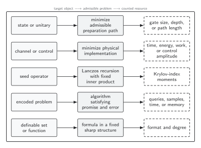
A complexity value is defined only after the target object selects an admissible family of paths or descriptions. Circuit length, physical control cost, Krylov spread, algorithmic resources, and sharp o-minimal format or degree answer different questions. The diagram is schematic and not to scale.

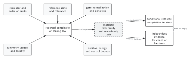
Reference sensitivity, gate nonuniqueness, regulator dependence, symmetry constraints, and unbounded controls are distinct failure modes. A link from complexity growth to chaos or computational hardness requires separate evidence after those controls. The diagram is schematic.

References

• Jefferson, Ro, and Robert C. Myers. “Circuit Complexity in Quantum Field Theory.” Journal of High Energy Physics 10 (2017): 107. DOI. Open PDF.
• Nielsen, Michael A. “A Geometric Approach to Quantum Circuit Lower Bounds.” Quantum Information & Computation 6 (2006): 213–262. Open PDF.