

Entanglement Growth after Quenches
After a quench, a subregion entropy can curve on the preparation scale, grow over an intermediate window, cross over when excitations resolve the whole region, and later feel the finite volume. The useful result is not merely that the curve rises. A publication-quality analysis identifies each regime in physical units, shows that the claimed window survives regulator and volume refinement, and explains which mechanism predicts its shape.
Required background. Equilibration and dephasing supplies the closed-system relaxation picture, closed-time-path evolution supplies real-time observables, and the quench contract fixes the regulated problem.
Helpful background. Thermal and excited-state entanglement supplies candidate equilibrium entropy densities, without assuming that every quench thermalizes to an ordinary Gibbs ensemble.
Reading an entropy curve
Section titled “Reading an entropy curve”For a region in a globally pure state, calculate
The subtraction cancels the state-independent leading divergence associated with the same entangling cut. It does not guarantee that all cutoff dependence has disappeared: a preparation that changes ultraviolet correlations can leave state-dependent terms, and an interacting calculation may require additional renormalized observables as cross-checks.
For a one-dimensional interval of length inside a much larger system, separate four candidate regimes:
- Preparation transient: is comparable with the ramp time, extrapolation length, inverse initial gap, or lattice scale. Curvature here is expected and is generally protocol dependent.
- Growth window: the region boundary receives correlated excitations from increasing distances. Linear growth is common in ballistic scaling regimes, but power laws, logarithms, and crossovers are also possible.
- Region-size crossover: the fastest relevant carriers have traversed a distance of order , and the leading extensive contribution approaches a plateau.
- Finite-system or numerical regime: boundary returns, recurrences, local-Hilbert-space truncation, or tensor-network bond limits alter the curve.
Those labels are hypotheses until scale variations identify them. Plotting against lattice time steps can make a cutoff transient appear to widen; plotting only against can hide a fixed physical preparation time. Show at least one panel or table in physical units before attempting a scaling collapse.
Conformal scaling benchmark
Section titled “Conformal scaling benchmark”A controlled analytic baseline comes from the boundary-state global quench of a one-dimensional conformal field theory. The regulated initial state is modeled as , and the long-distance observables correspond to an effective inverse temperature
For an interval of length on an infinite line, with , the leading extensive entropy is
The factor of two has a geometric meaning: an interval has two endpoints, and pairs produced within a distance of either endpoint can be shared across that cut. The crossover time is when the relativistic speed is one. Calabrese and Cardy 2005, §§ 2–4 derive the smooth finite- result whose scaling limit has this form.
For , , and , one obtains
These benchmark values belong to the displayed scaling approximation, not to a generic mass quench or to the rounded finite- answer. They are nevertheless valuable regression tests for factors of two, endpoint counting, and the conversion between and .
Local quenches grow differently
Section titled “Local quenches grow differently”A local quench changes the Hamiltonian or joins subsystems only near one position, so it injects a finite amount of energy rather than a finite energy density throughout space. In the conformal joining-quench benchmark, two initially disconnected half-lines are joined with a short-distance smoothing scale . For the half-line entropy,
At late time this grows logarithmically, not linearly, and there is no extensive interval plateau of the global-quench form. For , , and ,
This is an adversarial protocol check: code or prose that returns the global-quench value for this initial state has conflated two preparations. The regulated conformal joining calculation is derived by Calabrese and Cardy 2007, § 3.1.
Locality supplies an upper bound, not a universal growth law. For a finite-dimensional short-range lattice system, the entanglement-production rate can be bounded in terms of interactions crossing the boundary, and Lieb–Robinson estimates limit how quickly distant degrees of freedom can contribute Bravyi, Hastings, and Verstraete 2006, pp. 2–4. These hypotheses do not directly cover an untruncated bosonic site Hilbert space. Even where the bound applies, “at most linear” does not imply that the actual entropy is linear.
Free-scalar mass-quench extraction
Section titled “Free-scalar mass-quench extraction”For the Gaussian quench on the contract page, compute the full covariance entropy for several physical intervals , at multiple lattice spacings and volumes. A useful analysis proceeds in this order:
- At each , verify full-state purity, final energy conservation, and timestep convergence.
- At fixed physical , extrapolate the common-cut subtraction in .
- Increase until the first boundary-sensitive time lies beyond the proposed fit window.
- Estimate a local slope with several differentiation or regression windows.
- Freeze the fit rule, then compare all and predict their crossover times.
The scalar calculation is especially instructive because the exact covariance result and the independently constructed quasiparticle result can be compared without fitting an arbitrary slope. Cotler et al. 2016, §§ 3.1–3.3, pp. 15–24 find leading large-region agreement for free scalars while also identifying subleading zero-mode effects. The latter warn against reading a small residual logarithm as a failure of the leading ballistic picture.
Define a dimensionless effective slope only after choosing the equilibrium or stationary entropy density:
might be a Gibbs entropy density, a generalized-ensemble entropy density, or a directly measured late-time density. The choice is part of the result. A stable numerator combined with the wrong yields a precise but meaningless “velocity.”
Report sensitivity to the fit endpoints. If changes monotonically as is moved away from the transient, the asymptotic window has not yet been reached. If it changes when is increased but the fit time is held fixed, the assumed scale separation may be absent.
A controlled several-size mass quench
Section titled “A controlled several-size mass quench”The procedure above can be carried out without fitting an entropy slope. Consider the periodic canonical chain
Prepare the exact ground state at and switch suddenly to . The calculation shown below fixes and , so , and uses physical interval lengths
At every sampled time, Fourier-transform the analytic mode covariances from the quench contract, restrict them to the interval, and diagonalize the positive symplectic spectrum . The exact finite-lattice entropy is
The subtraction uses precisely the same lattice cut. No time integrator is involved: mode evolution is analytic, and is only the plotting and threshold-sampling interval. This distinction matters because the covariance contains frequencies up to . Here , so Nyquist sampling alone requires
The chosen sampling is about one quarter of that limit.
For a size-rescaled comparison, determine the post-quench mode occupation and stationary mode-entropy density rather than fitting a plateau:
The leading large-interval quasiparticle curve is then
with . This curve contains no fitted rate. It is the leading scaling comparison for this integrable quench, not an exact finite- identity; Alba and Calabrese 2017, Eqs. (2)–(3), pp. 7947–7949 give the mode-resolved integrable formula, and the following page derives the quasiparticle formula and its domain. Cotler et al. 2016, §§ 2.1–2.2 and 3.1–3.3, pp. 9–24 develop the exact Gaussian construction and compare free-scalar results with the large-region quasiparticle prediction; their reported comparison uses a massless post-quench scalar, whereas the benchmark here keeps .
Inspect both panels of the figure. The upper panel asks whether the several-size curves organize when time and entropy are scaled by . The lower panel repeats the calculation in a deliberately small ring and in a larger control ring, so the apparent growth law is tested against its own predicted finite-volume failure.
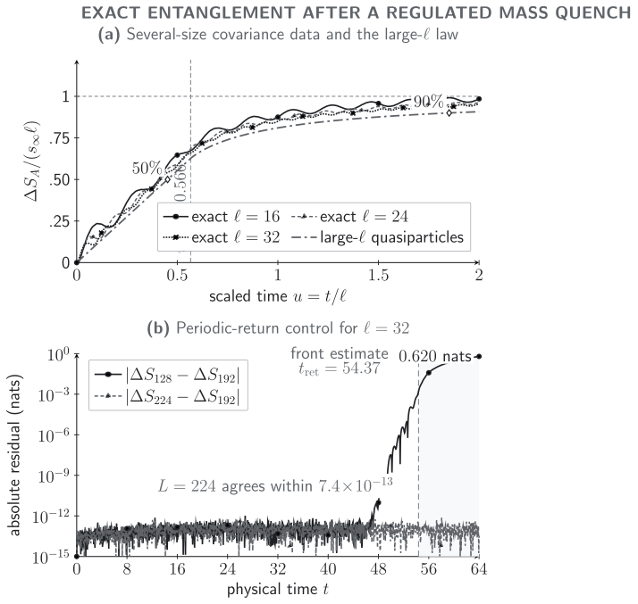
Several-size entropy growth and its volume control. For the exact periodic Gaussian quench at , the upper panel compares for with the parameter-free large- quasiparticle curve. The vertical line at marks the fastest-mode crossing, not saturation; slow modes produce the long approach to the leading stationary volume term. The lower panel shows the absolute residual relative to : the deliberately small ring departs near the front estimate and reaches nats by , whereas agrees within . The plot is quantitative, not schematic, and the return time is a front estimate rather than a strict zero-support theorem.
The subtracted entropy curves for all three intervals agree within through , which is half the fastest-carrier crossing time of the smallest interval. This is numerical evidence for a common early physical-time curve, not a proof of an exact light cone for an untruncated bosonic chain. After rescaling, the first crossings of one half of the leading volume term occur at
a spread of about . The thermodynamic-lattice quasiparticle curve reaches one half at and only at . Its largest group velocity is , so the fastest carriers begin the region-size crossover at
The ordering is important: marks the arrival of the fastest relevant modes, while slower modes continue adding entropy long afterward.
A naive “first crossing of ” rule would give , , and for the three exact curves. Those values do not collapse, and the quasiparticle curve has reached only , , and at the same scaled times. The exact-minus-leading difference is nearly size independent—about – nats—so an order-one coherent or boundary correction moves a fixed fractional threshold more strongly at smaller . Calling those crossings “saturation times” would turn a finite-interval correction into a false size dependence.
A straight-looking transient is not a velocity
Section titled “A straight-looking transient is not a velocity”The adversarial check deliberately ignores the full curve and fits only the preparation-scale transient. In each time window, use unweighted ordinary least squares with a free intercept,
The factor counts the two endpoints of a one-dimensional interval. The four adjacent windows below have width and contain 11 samples each. They all end by , well inside the numerically checked common-curve interval , so interval-size crossover cannot explain their disagreement.
| Time window | Entropy slope | ||
|---|---|---|---|
| – | |||
| – | |||
| – | |||
| – |
All three interval sizes reproduce these slopes within , including after serialization to the downloadable CSV, yet moving the window changes the proxy by more than two units and reverses its sign. Even the first two locally straight fits exceed the lattice carrier speed . This is not a causality violation: is an entropy slope divided by a chosen entropy density, not a measured signal speed, and a finite-subregion entropy need not increase monotonically during coherent unitary evolution. A large certifies local straightness, not the physical interpretation of the line.
The short-window velocity claim therefore fails. What survives is the parameter-free full-curve comparison, whose leading quasiparticle entropy velocity is , together with the several-size and regulator controls. The machine-readable record also gives every fit intercept and residual; those residuals diagnose curvature, not stochastic uncertainty.
The systematic controls set the claim boundary:
- The main curves stop at , before the earliest periodic-return estimate .
- Increasing the ring to changes the displayed curve by at most . Reducing it to deliberately violates the late-time volume window and produces the visible deficit.
- Repeating sampled checks at changes by at most of over the tested intervals and times. The benchmark is stable in this two-spacing sampled check and is consistent with cutoff convergence, but it is not a continuum extrapolation.
- Mode purity is preserved to , relative final-energy drift is , symplectic pairing closes within , and a no-quench control keeps . These are floating-point verification residuals, not physical error bars.
The strongest supported statement is consequently narrow and useful: at this regulator, the exact several-interval entropies share a common early curve and an approximately size-rescaled crossover before periodic return, with a slow-mode tail and visible order-one finite-interval corrections. The data do not establish a continuum entropy-production rate or a universal chaotic entanglement velocity. Download the quantitative SVG, the complete CSV curve and residual data, and the JSON calculation, controls, and claim boundary.
What a plateau does and does not mean
Section titled “What a plateau does and does not mean”For a small region in a very large, locally equilibrated system, a volume-law plateau can agree with a thermal or generalized-equilibrium entropy density even though the global state remains pure. The complement purifies the region. For a finite pure system,
so an interval larger than half the system cannot follow a naive law; its leading plateau is controlled by the smaller side. Page-curve corrections and exact constraints can matter near half system.
Integrable systems may relax locally to a generalized Gibbs ensemble whose thermodynamic entropy supplies the quasiparticle weights Alba and Calabrese 2017, pp. 7947–7949. Chaotic systems can display a thermal entropy density but still have long hydrodynamic tails. A localized system may not reach a volume-law thermal plateau on accessible times. Thus saturation is a geometric feature of a finite region; thermalization is an independent statement about the reduced state and its observables.
A numerical plateau requires its own controls. In a matrix-product-state calculation, insufficient bond dimension caps the entropy at approximately . Increase until the plateau position and height stop moving. In a bosonic truncation, increase the local occupation cutoff and verify both energy and covariance tails. In exact diagonalization, move and the region together so that a finite-size plateau is not confused with the thermodynamic one.
Reproducible curve-to-claim workflow
Section titled “Reproducible curve-to-claim workflow”For every candidate growth law, publish or retain enough information to reconstruct the inference:
- raw or finite-difference data with numerical uncertainty;
- the subtraction and the same-cut geometry used at ;
- the physical transient exclusion criterion;
- at least three interval sizes and two larger volumes;
- regulator and timestep convergence at representative early, fit-window, and plateau times;
- fit residuals for linear and plausible competing forms;
- the independently determined ;
- an out-of-sample prediction, such as a new interval or initial state.
The chapter orientation map distinguishes this direct curve from the effective picture used to explain it. Apply the independent failure controls, and use the diagnostic comparison before calling an entropy slope a transport speed.
Common pitfalls
Section titled “Common pitfalls”Fitting the first straight-looking segment. A smooth transient can look linear over less than a decade. Move both fit endpoints, refine the preparation scale, and require a window that widens in physical units.
Comparing raw entropies across cutoffs. The leading divergence changes with . Use a same-geometry subtraction or a finite information measure and still demonstrate residual convergence.
Calling every plateau thermal. Purity, finite region size, bond dimension, localization, and generalized equilibrium can all produce plateaus or slowdowns. Compare the reduced state with the claimed ensemble and vary the numerical ceiling.
Exercises
Section titled “Exercises”For the conformal benchmark with arbitrary , , and , show that the early linear branch meets the plateau at .
Solution
The early branch is . At it equals
which is the plateau value. The equality is independent of and because both branches contain the same entropy density. Finite rounds the meeting point rather than creating a discontinuity in the derivative of the exact answer.
A tensor-network run shows an entropy plateau at for bond dimension . Compare this value with the maximum Schmidt entropy using natural logarithms. What conclusion is justified?
Solution
Since
the observed plateau lies close to the absolute bond-dimension ceiling. It may be truncation rather than physical saturation. The run alone supports no thermalization claim; increase , inspect discarded weight, and verify that the plateau time and height converge.
Suppose a linear fit gives slopes , , and when the lower endpoint is moved from to to , while the upper endpoint remains . A separate refinement moves the preparation time from to . Explain why quoting the first slope as an asymptotic rate is unjustified and propose a better test.
Solution
The systematic decrease with shows that the fit is resolving curvature. Moreover, the preparation scale can occupy much of the window. A better test holds the preparation protocol fixed in physical units, increases both the interval and the volume, and searches for a range with and over which the local derivative and regression slope agree and remain stable as both endpoints move.
References
Section titled “References”- Alba, Vincenzo, and Pasquale Calabrese. “Entanglement and Thermodynamics after a Quantum Quench in Integrable Systems.” Proceedings of the National Academy of Sciences 114 (2017): 7947–7951. DOI.
- Calabrese, Pasquale, and John Cardy. “Evolution of Entanglement Entropy in One-Dimensional Systems.” Journal of Statistical Mechanics: Theory and Experiment 2005 (2005): P04010. DOI.
- Calabrese, Pasquale, and John Cardy. “Entanglement and Correlation Functions Following a Local Quench: A Conformal Field Theory Approach.” Journal of Statistical Mechanics: Theory and Experiment 2007 (2007): P10004. DOI.
- Bravyi, Sergey, Matthew B. Hastings, and Frank Verstraete. “Lieb–Robinson Bounds and the Generation of Correlations and Topological Quantum Order.” Physical Review Letters 97 (2006): 050401. DOI.
- Cotler, Jordan S., Mark P. Hertzberg, Márk Mezei, and Mark T. Mueller. “Entanglement Growth after a Global Quench in Free Scalar Field Theory.” Journal of High Energy Physics 2016, no. 11 (2016): 166. DOI.