

Path-Integral and Euclidean Preparation Complexity
A Euclidean path integral can specify a state-preparation map once its boundary data, sources, geometry, regulator, and normalization are fixed. It does not by itself assign a complexity. A cost arises only after declaring which deformations or discretized tensors are admissible and what resource they consume. Action value, optimized geometry, tensor count, and real-time circuit depth are distinct proposals.
Required background. Circuit Complexity in Quantum Field Theory supplies the regulated preparation task.
Helpful background. Replica Trick and Branched Geometries supplies the geometric and analytic-continuation discipline needed when Euclidean manifolds are cut or branched.
Euclidean evolution prepares a boundary wavefunctional
Section titled “Euclidean evolution prepares a boundary wavefunctional”For a scalar field, a vacuum wavefunctional may be represented schematically as
More generally, sources , an Euclidean metric, boundary terms, and operator insertions prepare a family of states. This formula specifies amplitudes after a regulator and renormalization prescription are supplied. It is neither a normalized physical probability distribution over histories nor a unitary circuit in Lorentzian time.
Discretize Euclidean time into steps . Each factor is nonunitary and suppresses excited states. A unitary laboratory implementation needs dilation, postselection, cooling, or another channel model, whose success probability and resources must be charged. Counting Euclidean layers therefore measures a representation or imaginary-time algorithm, not automatically physical duration.
Three resource models
Section titled “Three resource models”Discretized transfer resource. Fix a spatial regulator and approximate by a product formula or tensor network. Count tensors, bond dimensions, arithmetic operations, or approximation error. The algorithmic implementation is developed in Volume 8; here the issue is the QFT target and the continuum comparison. A path-integral geometry can organize a tensor-network representation, but the representation is not thereby a minimal physical circuit Milsted and Vidal 2018, §§2–4.
Source-and-geometry cost. Choose allowed and Euclidean geometries , then minimize a functional subject to preparing the target. This is a proposal whose coordinate, Weyl, boundary, and counterterm dependence must be stated. Path-integral optimization in two-dimensional CFT provides an influential example, but its Liouville-type objective is not a definition for all QFTs Caputa et al. 2017, §§2–4.
Circuit translation. Construct an explicit channel or circuit that approximates the discretized transfer map on a declared energy subspace. Then compare its gate or control cost with the Euclidean description. This direction can establish an upper bound; equality requires an optimality theorem.
Gaussian preparation as a controlled example
Section titled “Gaussian preparation as a controlled example”For a regulated free mode of frequency , propagation over Euclidean time suppresses the th excitation by . Starting from a reference with nonzero vacuum overlap, the normalized state approaches the vacuum with error controlled by , where is the relevant gap. At finite volume one can choose to meet a fidelity tolerance.
A reproducible comparison evaluates:
- Euclidean step count and Trotter error;
- tensor rank or bond resource after spatial discretization;
- a unitary or dissipative implementation cost with success probability;
- the Gaussian circuit cost for the same target, reference, and tolerance.
Refining increases representation size without changing the physical target. A cost that grows only because a coordinate mesh was refined is discretization complexity unless an invariance or renormalization rule removes that dependence.
Reparameterization and counterterms
Section titled “Reparameterization and counterterms”Under , the same Euclidean region can acquire a different coordinate thickness and source profile. Any proposed integral density must transform so the total has the intended invariance. Boundary and local ultraviolet counterterms can shift action-like values. Report which terms are fixed by state normalization, which are allowed preparation costs, and which remain scheme dependent.
As of 10 August 2026, Euclidean path-integral costs are a family of definition-dependent constructions, not an experimentally established universal QFT complexity. Their strongest use is as controlled preparation descriptions and comparisons within a fixed proposal.
Exercises
Section titled “Exercises”Mesh refinement. A cost equals the number of Euclidean time slices. What happens under at fixed ?
Solution
The count doubles although the exact transfer operator is unchanged. This is a discretization resource. A physical comparison must include the approximation error and either optimize the mesh or translate the slices into a charged implementation.
Gapless limit. Why does the simple preparation estimate fail in infinite-volume massless QFT?
Solution
The spectral gap closes, so no uniform finite suppresses all low-energy excitations. One must specify finite volume, an energy or observable tolerance, or another preparation protocol and control the order of limits.
Task and validity maps
Section titled “Task and validity maps”The first diagram distinguishes target objects and their admissible resource models; inspect which equivalence class is being minimized over. The second shows the definition changes and physical controls that must be held fixed before two complexity values or growth laws are compared.
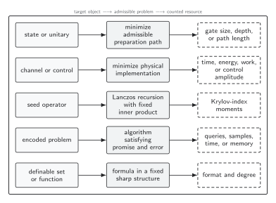
A complexity value is defined only after the target object selects an admissible family of paths or descriptions. Circuit length, physical control cost, Krylov spread, algorithmic resources, and sharp o-minimal format or degree answer different questions. The diagram is schematic and not to scale.
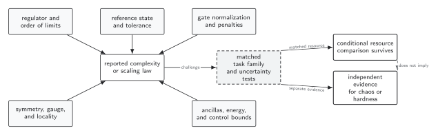
Reference sensitivity, gate nonuniqueness, regulator dependence, symmetry constraints, and unbounded controls are distinct failure modes. A link from complexity growth to chaos or computational hardness requires separate evidence after those controls. The diagram is schematic.
References
Section titled “References”- Caputa, Paweł, Nilay Kundu, Masamichi Miyaji, Tadashi Takayanagi, and Kento Watanabe. “Liouville Action as Path-Integral Complexity: From Continuous Tensor Networks to AdS/CFT.” Physical Review Letters 119 (2017): 071602. DOI. Open PDF.
- Milsted, Ashley, and Guifré Vidal. “Tensor Networks as Path Integral Geometry.” arXiv:1807.02501 (2018). Preprint.