Correlation-Matrix and Gaussian-State Reconstruction

Measured one- and two-point functions determine a bosonic or fermionic Gaussian state once the physical mode algebra and normalization are fixed. Reconstruction therefore has two logically separate parts: certify that the estimated covariance is physical, then state the evidence that the actual state is Gaussian. The first is a matrix constraint; the second is a model-validation problem.

Required background. From Field Data to Information Claims supplies calibration and uncertainty. Gaussian States and Correlation-Matrix Entropy supplies covariance conventions.

Helpful background. Entropy and Rényi Estimation Protocols supplies downstream estimator checks.

Bosonic physicality and estimation

For quadratures $R=(q_1,p_1,\ldots,q_m,p_m)^T$ with $[R_j,R_k]=i\Omega_{jk}$ , estimate the mean $d=\langle R\rangle$ and covariance

V_{jk}=\frac12\langle\{R_j-d_j,R_k-d_k\}\rangle.

A physical covariance satisfies

V+\frac{i}{2}\Omega\geq0.

An unconstrained sample covariance can violate this inequality because of noise or miscalibration. Projecting to the nearest physical covariance changes the estimator and introduces bias. Prefer a constrained likelihood or estimating equation when possible; otherwise record the projection metric and propagate it inside resampling.

Symplectic eigenvalues $\nu_k\geq1/2$ determine the entropy in this convention. Near $\nu_k=1/2$ , nonlinear uncertainty and the physical boundary make symmetric error bars unreliable.

Fermionic covariance

For Majorana operators $\gamma_j$ with $\{\gamma_j,\gamma_k\}=2\delta_{jk}$ , estimate

\Gamma_{jk}=\frac{i}{2}\langle[\gamma_j,\gamma_k]\rangle, \qquad \Gamma^T=-\Gamma, \qquad \lVert\Gamma\rVert\leq1.

Parity superselection and mode ordering are part of the reconstruction. A Gaussian fermionic state is fixed by $\Gamma$ within a declared parity sector; an arbitrary state with the same $\Gamma$ is not.

Noisy squeezed-thermal benchmark

Generate a multimode squeezed thermal state and simulate calibrated quadrature measurements. Fit $d,V$ under the physicality constraint. For each bootstrap or posterior draw:

sample raw records and calibration parameters jointly;
refit the physical covariance;
compute symplectic eigenvalues and entropy;
record fit residuals and held-out quadratures.

Then create a non-Gaussian mixture with matching $d,V$ . Covariance-based entropy returns the entropy of the corresponding Gaussian state, not necessarily the mixture’s entropy. Measure selected fourth cumulants or compare a direct purity estimator to challenge Gaussianity. A null result has finite power and should bound, not eliminate, non-Gaussian alternatives.

Mode completeness and continuum bias

Reconstruction is only for the measured wave-packet or truncated mode algebra. Missing modes can be correlated with the retained ones, making the reduced state mixed. State the mode functions, orthogonality calibration, energy cutoff, and leakage. Increasing the number of modes changes the target state space, so uncertainty and continuum extrapolation must be repeated rather than appended afterward.

Systematic tomography biases can make physical-looking reconstructions inconsistent with the true measurement model Schwemmer et al. 2015, pp. 1–4. Held-out outcomes and residual structure are therefore mandatory.

Exercises

Projection bias. Why can clipping a symplectic eigenvalue to $1/2$ understate entropy uncertainty?

Solution

It piles noisy estimates on the physical boundary and makes the transformed distribution non-Gaussian. Refit or reproject within every resample and report asymmetric intervals and boundary frequency.

Same covariance. What claims survive when a non-Gaussian alternative matches $d,V$ ?

Solution

All measured first and second moments, covariance witnesses valid for arbitrary states, and properties of the maximum-entropy Gaussian state survive. Exact state reconstruction and entropy of the unknown state do not.

Inference and failure-control maps

The first diagram traces the complete path from raw records to a bounded information claim; inspect the assumption attached to every arrow. The second maps shared and method-specific failure channels to held-out tests, regulator variation, replication, and correction.

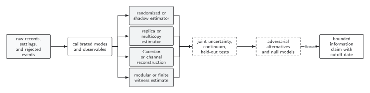
Raw field or simulator records pass through calibration, an estimator and model, correlated uncertainty, continuum checks, and adversarial alternatives before a bounded information claim is issued. — Entropy, tomography, witness, and recovery methods enter at the estimator stage, but all share calibration, uncertainty, continuum, and alternative-model tests. The final statement is no stronger than the least validated arrow. The diagram is schematic and not to scale.

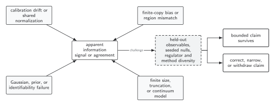
Calibration drift, finite copies, model mismatch, continuum extrapolation, and shared normalization can all imitate an information signal; held-out tests, method diversity, replication, and correction constrain them. — Different estimators can share the same calibration or normalization bias, so numerical agreement is not automatically independent replication. Adversarial nulls, held-out observables, regulator variation, and genuinely independent implementations set the claim ceiling and trigger correction when needed. The diagram is schematic.

References

Schwemmer, Christian, Lukas Knips, Daniel Richart, Harald Weinfurter, Tobias Moroder, Matthias Kleinmann, and Otfried Gühne. “Systematic Errors in Current Quantum State Tomography Tools.” Physical Review Letters 114 (2015): 080403. DOI. Open PDF.