

Gaussian-State Complexity
Gaussian states make QFT circuit complexity calculable because a state is fixed by first and second moments and Gaussian gates act linearly on canonical variables. The answer still depends on the reference covariance, the allowed symplectic or orthogonal transformations, the cost, and the regulator. Bosonic and fermionic formulas look parallel but live on different groups and require different treatments of zero modes and parity.
Required background. Cost Geometry, Gate Sets, and Reference States supplies the geometric minimization.
Helpful background. Gaussian States and Correlation-Matrix Entropy supplies covariance conventions and mode diagnostics.
Bosonic covariance geometry
Section titled “Bosonic covariance geometry”Collect bosonic modes into with . For vanishing mean, the covariance is
A Gaussian unitary acts by , so . Given pure reference and target covariances , the relative matrix
encodes the required squeezing. In a standard unpenalized quadratic geometry, a representative geodesic is generated by , and the cost is a chosen norm of . The numerical prefactor changes with covariance and generator normalization, so both must accompany the result.
Displacements add a semidirect-product sector. Ignoring a nonzero mean can incorrectly declare two coherent states equally complex. A massless zero mode has divergent position variance in finite volume unless the state, boundary condition, or infrared regulator is specified. The regulated free-field construction and its reference dependence are worked out by Jefferson and Myers 2017, §§2–4.
Fermionic covariance geometry
Section titled “Fermionic covariance geometry”For Majorana operators with , define
Pure Gaussian states satisfy , and parity-preserving Gaussian unitaries act by : . Relative complex structures determine rotation angles rather than unbounded squeeze parameters. Gate paths must remain in the admissible parity component; allowing an orientation-reversing orthogonal map can connect states that physical even gates cannot.
Circuit complexity for free fermions is developed with these relative-covariance methods by Hackl and Myers Hackl and Myers 2018, §§2–4. Bosonic and fermionic values should be compared only after matching the cost normalization and number of independent modes.
Mass-quench example
Section titled “Mass-quench example”Regulate a scalar field so that each momentum mode has frequency
where is the regulator dispersion. Preparing the vacuum from the vacuum by modewise squeezing requires
For an norm, ; for , . To study a real-time quench rather than ground-state conversion, evolve the covariance with the post-quench symplectic matrix and recompute the relative matrix at each time. Report whether the circuit is allowed to use momentum-space nonlocal gates or only spatially local ones.
For a fermionic mass quench, Bogoliubov angles replace . Matching a bosonic and a fermionic study requires the same physical volume, momentum convention, fidelity or covariance error, degeneracy counting, and ultraviolet cutoff—not merely the same number of lattice sites.
Independent checks
Section titled “Independent checks”- Verify for bosons or for fermions.
- Apply the proposed transformation and compare the resulting moments with the target.
- Check symplectic or orthogonal constraints numerically.
- isolate zero modes and degeneracies before summing.
- vary the reference frequency and gate penalty to expose conventional pieces.
- refine the regulator at fixed physical mass, volume, and target error.
Gaussian solvability controls the optimization only within the Gaussian gate class. A shorter non-Gaussian path may exist unless it is excluded by the task.
Exercises
Section titled “Exercises”Reference sensitivity. For one bosonic mode, show that changing shifts the squeeze coordinate.
Solution
The coordinate is . Replacing by gives . The state is unchanged; the preparation task and its cost changed.
Fermionic component. Why must parity be included in the gate specification?
Solution
Even quadratic generators produce transformations in the connected parity-preserving component. An arbitrary orthogonal transformation can change the component and may require a parity-odd operation. Minimizing over it would solve a larger, unphysical gate problem.
Task and validity maps
Section titled “Task and validity maps”The first diagram distinguishes target objects and their admissible resource models; inspect which equivalence class is being minimized over. The second shows the definition changes and physical controls that must be held fixed before two complexity values or growth laws are compared.
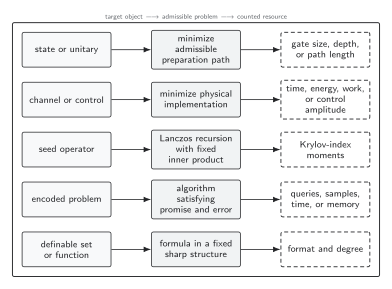
A complexity value is defined only after the target object selects an admissible family of paths or descriptions. Circuit length, physical control cost, Krylov spread, algorithmic resources, and sharp o-minimal format or degree answer different questions. The diagram is schematic and not to scale.
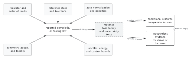
Reference sensitivity, gate nonuniqueness, regulator dependence, symmetry constraints, and unbounded controls are distinct failure modes. A link from complexity growth to chaos or computational hardness requires separate evidence after those controls. The diagram is schematic.