Complexity, Chaos, and Computational Claims

Complexity growth, chaos, and computational hardness are separate claims. Circuit complexity concerns a chosen synthesis task; Krylov complexity concerns a chosen operator basis; chaos concerns dynamical sensitivity or spectral correlations; computational hardness concerns families of encoded problems. Evidence for one can motivate a comparison with another, but no generic implication follows in QFT.

Required background. Lyapunov Growth and Chaos Bounds supplies the hypotheses behind regulated exponential growth. What Task Does Complexity Answer? supplies the resource distinctions.

Helpful background. Krylov and Operator-Growth Complexity supplies the Lanczos construction, and Scrambling Evidence and Claim-Status Matrix supplies matched alternatives and evidence ceilings.

A claim matrix, not a chain of synonyms

Observed quantity	Direct claim	Needed for a stronger claim	Counterexample strategy
minimal circuit cost grows	target becomes costly in a fixed gate model	gate robustness and physical implementation	choose an easy target in a chaotic system
Krylov moment grows	seed spreads in one Lanczos basis	seed and inner-product robustness plus independent chaos test	use a free or integrable model with rapid Krylov growth
regulated OTOC grows or decays	selected operators develop influence	connected normalization, contour, sectors, finite-size controls	use decoherence or a restricted operator family
Wigner–Dyson statistics	level correlations in a resolved finite spectrum	unfolding and symmetry controls; dynamical evidence	mix unresolved symmetry sectors
simulation runtime is large	one algorithm or instance family is costly	lower bound in a stated computational model	change encoding, oracle, or observable
holographic proposal grows	one bulk prescription has stated behavior	an independent field-theory task and duality dictionary	compare inequivalent boundary costs

The matrix blocks two common invalid inferences:

$$\text{growing chosen complexity}\not\Rightarrow\text{chaos}, \qquad \text{chaos}\not\Rightarrow\text{hard preparation of every target}.$$

Matched integrable and chaotic comparisons

A useful numerical study selects regulated integrable, chaotic, and free models with matched Hilbert dimension, energy density, symmetries, and operator normalization. For each model compute:

1. level statistics within irreducible symmetry sectors;
2. a regulated OTOC or commutator over a controlled time window;
3. Lanczos coefficients and $K(t)$ for several seeds and inner products;
4. a circuit or control upper bound for the same declared target family;
5. finite-size, time-window, and cutoff convergence.

The comparisons should include null targets. The time-evolved state $e^{-iHt}|\psi_0\rangle$ may be cheap when the gate set contains the Hamiltonian evolution, even if other synthesis models call it costly. Conversely, a nonchaotic free field can require many local gates to prepare a long-range-correlated state.

Parker and collaborators propose asymptotic operator-growth constraints under locality assumptions Parker et al. 2019, §§II–IV. Later QFT analyses find substantial mass, volume, seed, and ultraviolet sensitivity Avdoshkin, Dymarsky, and Smolkin 2024, §§3–6. These results support careful conditional comparisons, not a universal identification of Krylov and chaos exponents.

Computational claims require reductions

To say that estimating a QFT observable is hard, specify an input encoding, problem size $n$, promise gap, desired error, success probability, and classical or quantum computational model. Then prove a lower bound or a reduction from a recognized hard problem. The empirical failure of one optimizer supplies an algorithm benchmark, not a complexity-class result.

Circuit-geometric complexity also differs from computational gate complexity. A continuous geometry can charge an analog parameter by its path length while ignoring bits of precision; an algorithm must encode that parameter. Conversely, an oracle query can have unit computational cost while representing an expensive physical operation.

Holographic and conjectural boundaries

Bulk action, volume, or spacetime prescriptions belong to the holographic volume. If used as evidence here, the page must state the duality setting, boundary state, normalization, regulator dictionary, and which independently defined field-theory task is compared. Qualitative linear growth in two proposals does not establish equality.

As of 10 August 2026, the defensible general statement is negative but useful: no known definition-independent complexity growth law characterizes chaos or computational hardness across QFTs. Model-specific correlations can be strong and scientifically informative when the task tuple and independent diagnostics are complete.

Adversarial examples

Growing complexity without chaos. A free-field vacuum prepared from an unentangled lattice reference has a circuit cost that grows with the number of modes. This ultraviolet growth reflects the target correlations and gate model, not chaotic dynamics.

Chaos with an easy target. In a chaotic regulated Hamiltonian, the identity channel, an eigenstate supplied as the reference, or evolution generated by a gate primitive can have trivial cost for its declared task. Chaos is a property of wider dynamics, not a lower bound for every synthesis problem.

Apparent hardness without a lower bound. A variational optimizer can stall because of poor parameterization or conditioning while a different algorithm succeeds. Runtime evidence must compare algorithms and instances before any hardness conjecture is stated.

Exercises

One-way evidence. A model has Wigner–Dyson statistics and a rapidly growing $K(t)$ for one seed. What can be claimed?

Solution

Within the resolved finite system, two diagnostics are consistent with chaotic spectral behavior and rapid spreading of that seed in that inner product. One cannot infer universal circuit growth, computational hardness, recoverability loss, or a continuum exponent without the corresponding tasks and controls.

Gate-set reversal. Explain how adding exact time evolution $e^{-iH\delta t}$ as a primitive changes preparation complexity.

Solution

The evolved state can be prepared in $t/\delta t$ primitive steps, or one step if arbitrary $t$ is a free parameter. The physical dynamics is unchanged; the synthesis resource changed. Any chaos–complexity comparison must therefore fix and justify the gate model.

Task and validity maps

The first diagram distinguishes target objects and their admissible resource models; inspect which equivalence class is being minimized over. The second shows the definition changes and physical controls that must be held fixed before two complexity values or growth laws are compared.

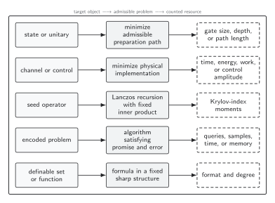
A complexity value is defined only after the target object selects an admissible family of paths or descriptions. Circuit length, physical control cost, Krylov spread, algorithmic resources, and sharp o-minimal format or degree answer different questions. The diagram is schematic and not to scale.

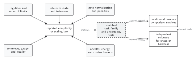
Reference sensitivity, gate nonuniqueness, regulator dependence, symmetry constraints, and unbounded controls are distinct failure modes. A link from complexity growth to chaos or computational hardness requires separate evidence after those controls. The diagram is schematic.

References

• Avdoshkin, Alexander, Anatoly Dymarsky, and Michael Smolkin. “Krylov Complexity in Quantum Field Theory, and Beyond.” Journal of High Energy Physics 06 (2024): 066; corrected arXiv version 2025. DOI. Open PDF.
• Parker, Daniel E., Xiangyu Cao, Alexander Avdoshkin, Thomas Scaffidi, and Ehud Altman. “A Universal Operator Growth Hypothesis.” Physical Review X 9 (2019): 041017. DOI. Open PDF.