Interacting-Field Complexity

Beyond Gaussian QFT, complexity is usually estimated with perturbative circuits, variational ansätze, effective descriptions, or numerical optimal control. These methods define useful regulated comparisons only when the state error, truncation order, renormalization conditions, and ansatz bias are controlled. An interacting correction to a chosen cost is not a universal observable of the fixed point.

Required background. Circuit Complexity in Quantum Field Theory supplies the regulated gate task.

Helpful background. Gaussian-State Complexity supplies the solvable reference around which the expansion is organized.

Perturbing the state and the circuit

For a regulated Hamiltonian

$$H(\lambda)=H_0+\lambda V+\delta H(\lambda,\Lambda),$$

let $|\Omega(\lambda)\rangle$ be the normalized ground state in a declared finite volume and symmetry sector. Perturbation theory gives

$$|\Omega(\lambda)\rangle =|0\rangle -\lambda\sum_{n\neq0} \frac{\langle n|V+\delta H_1|0\rangle}{E_n-E_0}|n\rangle +O(\lambda^2).$$

The circuit ansatz must be able to generate the correction. One may write

$$U(\lambda)=U_G\exp[-i\lambda K_1-i\lambda^2K_2+\cdots],$$

where $U_G$ prepares the Gaussian reference and $K_j$ contains allowed non-Gaussian generators. Matching the target state through order $\lambda^p$ gives an admissible upper bound on complexity. It does not prove global minimality, and its state error is $O(\lambda^{p+1})$ only if gaps, volume factors, and operator norms remain controlled.

This expansion uses the same reference-state, gate-set, and cost choices that already make the Gaussian answer definition dependent Jefferson and Myers 2017, §§2–4. Interactions add truncation and renormalization errors; they do not remove those choices.

Counterterms are part of the target Hamiltonian. Comparing two cutoffs while holding bare parameters fixed changes the physical theory; a continuum study instead fixes renormalized masses and couplings through stated conditions.

Variational and effective constructions

A variational family $|\psi(\theta)\rangle=U(\theta)|\Omega_R\rangle$ can be optimized by energy, fidelity to a benchmark, or projected residual

$$R(\theta)=\lVert(H-E(\theta))|\psi(\theta)\rangle\rVert.$$

Small energy error alone need not imply high fidelity when the gap is small. When a spectral gap $\Delta>0$ is known, an energy excess can bound excited-state weight; otherwise report the residual and observable errors directly. Complexity evaluated on the optimized ansatz is an upper bound within that gate family.

Effective circuits obtained by integrating out modes require a matching map. A simpler low-energy state can hide the cost of preparing the effective degrees of freedom or implementing the renormalization transformation. State which part is charged and which observables define the tolerated error.

Weakly interacting scalar example

For regulated $\lambda\phi^4$ theory, choose a Gaussian reference with a renormalized trial mass and add quartic generators compatible with translation and reflection symmetry. A controlled calculation should:

1. fix volume, cutoff, boundary conditions, and renormalization scheme;
2. tune counterterms to matched physical conditions;
3. solve the perturbative or variational state problem;
4. synthesize an admissible circuit and compute its cost;
5. compare against exact diagonalization at small mode number or an independent observable benchmark;
6. vary generator truncation, coupling, and cutoff.

Bhattacharyya, Shekar, and Sinha construct Nielsen-geometric estimates for interacting scalar theories and explicitly encounter perturbative breakdown regimes Bhattacharyya, Shekar, and Sinha 2018, §§2–5. Their result is evidence for that specified construction, not a unique interacting-QFT complexity.

Error statement and evidence ceiling

As of 10 August 2026, no generally accepted gate-and-cost prescription makes interacting continuum-QFT circuit complexity regulator independent. The strongest defensible output of a finite calculation is therefore a conditional statement of the form

$$C_{\mathcal G,F,\Lambda}^{(p)} =C_G+\sum_{j=1}^{p}\lambda^j c_j +O_{\mathcal D}(\lambda^{p+1}) +\delta_{\rm opt}+\delta_{\rm num},$$

with the domain $\mathcal D$, truncation estimate, optimizer residual, and numerical convergence supplied. Scheme variation belongs in the uncertainty or in a comparison table; it should not be erased by selecting the most favorable reference.

Common pitfalls

Using the free-state overlap as an error bar. An overlap computed in a truncated basis misses omitted high-energy states. Bound or vary the truncation and check local observables.

Inferring an RG monotone. A decrease along one flow can result from reference, cost, or cutoff conventions. Monotonicity needs a theorem for a fixed task family, not a plot from one ansatz.

Exercises

Gap dependence. Why does small energy error fail to guarantee high fidelity near a critical point?

Solution

The usual bound divides the energy excess by the gap. As the gap closes, a state can carry substantial weight in low-lying excited states while changing the energy only slightly. One needs direct state or observable error controls and finite-size scaling.

Scheme test. What must remain fixed when comparing the $O(\lambda)$ cost at two lattice spacings?

Solution

Match physical volume, renormalized mass and coupling, target observables, reference family, gate normalization, cost, and approximation tolerance. Retune bare parameters and counterterms at each cutoff.

Task and validity maps

The first diagram distinguishes target objects and their admissible resource models; inspect which equivalence class is being minimized over. The second shows the definition changes and physical controls that must be held fixed before two complexity values or growth laws are compared.

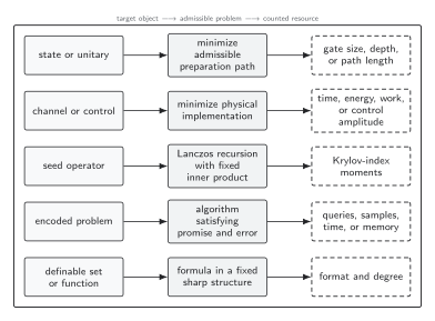
A complexity value is defined only after the target object selects an admissible family of paths or descriptions. Circuit length, physical control cost, Krylov spread, algorithmic resources, and sharp o-minimal format or degree answer different questions. The diagram is schematic and not to scale.

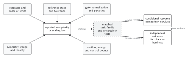
Reference sensitivity, gate nonuniqueness, regulator dependence, symmetry constraints, and unbounded controls are distinct failure modes. A link from complexity growth to chaos or computational hardness requires separate evidence after those controls. The diagram is schematic.

References

• Bhattacharyya, Arpan, Arvind Shekar, and Aninda Sinha. “Circuit Complexity in Interacting QFTs and RG Flows.” Journal of High Energy Physics 10 (2018): 140. DOI. Open PDF.
• Jefferson, Ro, and Robert C. Myers. “Circuit Complexity in Quantum Field Theory.” Journal of High Energy Physics 10 (2017): 107. DOI. Open PDF.