Equilibration, Thermalization, and Dephasing

Dephasing suppresses off-diagonal contributions to selected observables; equilibration means that those observables remain close to a stationary value for most times; thermalization further identifies that value with an ensemble fixed by the conserved data. Hydrodynamization and kinetic relaxation are still narrower statements about effective equations and quasiparticle distributions. None of them requires the exact finite-system density operator to converge.

Required background. Hilbert positivity and unitary evolution supplies spectral evolution and recurrence. Causal and statistical propagators supplies the observable two-point functions used in field theory. Helpful background. The H-theorem explains the stronger assumptions behind monotone kinetic entropy.

Observable relaxation under unitary evolution

Let a regulated isolated system have energy eigenstates $\lvert n\rangle$ and an initial state

$$\lvert\psi_0\rangle=\sum_n c_n\lvert n\rangle, \qquad p_n=\lvert c_n\rvert^2.$$

For a bounded observable $A$,

$$\langle A(t)\rangle =\sum_n p_nA_{nn} +\sum_{m\ne n}c_m^*c_nA_{mn}e^{i(E_m-E_n)t}.$$

If energy degeneracies are resolved within the relevant symmetry sector, the infinite-time mean is

$$\overline{\langle A\rangle} =\operatorname{Tr}(\omega A), \qquad \omega=\sum_n p_n\lvert n\rangle\langle n\rvert.$$

The diagonal ensemble $\omega$ is fixed by all populations $p_n$. Dephasing is the cancellation of the remaining oscillatory sum over many gaps. It is a mechanism, not an ensemble-identification theorem.

For nondegenerate energy gaps, the temporal variance is

$$\overline{\bigl\lvert\langle A(t)\rangle -\operatorname{Tr}(\omega A)\bigr\rvert^2} =\sum_{m\ne n}p_mp_n\lvert A_{mn}\rvert^2.$$

This formula exposes the ingredients of equilibration: many populated levels, sufficiently small off-diagonal matrix elements, and no extensive family of resonant gaps. More general bounds express the suppression through the effective dimension $d_{\mathrm{eff}}=(\sum_np_n^2)^{-1}$ Reimann 2008 and through subsystem dimension relative to $d_{\mathrm{eff}}$ Linden et al. 2009.

Six distinct claims

Claim	Object compared	Necessary declaration	Characteristic failure
Dephasing	off-diagonal phases in $\langle A(t)\rangle$	spectrum, initial amplitudes, observable	commensurate or degenerate gaps
Observable equilibration	$\langle A(t)\rangle$ versus a stationary value	tolerance and time window	large temporal variance or frequent revivals
Local equilibration	reduced state or local operator algebra	subsystem and norm/observable class	subsystem comparable with total system
Kinetic relaxation	$f(X,p)$ versus a kinetic fixed point	shell, gradient, collision assumptions	coherent, off-shell, or memory effects
Hydrodynamization	stress/current evolution versus constitutive theory	slow variables and gradient error	nonhydrodynamic modes remain large
Thermalization	stationary local data versus Gibbs/GGE data	conserved charges and ensemble	diagonal data retain additional memory

Isotropization is another independent comparison among spatial components. A stress tensor can satisfy hydrodynamics while its longitudinal and transverse pressures remain unequal, and a local observable can equilibrate without any quasiparticle description.

A state that never converges while observables equilibrate

For the pure state $\rho(t)=\lvert\psi(t)\rangle\langle\psi(t)\rvert$, compare it with its diagonal ensemble using the Hilbert–Schmidt norm. Directly,

$$\begin{aligned} \operatorname{Tr}\bigl[(\rho(t)-\omega)^2\bigr] &=\operatorname{Tr}\rho(t)^2+\operatorname{Tr}\omega^2 -2\operatorname{Tr}[\rho(t)\omega]\\ &=1-\sum_n p_n^2 =1-\frac1{d_{\mathrm{eff}}}. \end{aligned}$$

It is constant and nonzero whenever more than one energy is populated. Thus the full state does not approach $\omega$ even though the variance of every chosen few-body observable may be extremely small. The apparent irreversibility lies in restricting the observable algebra and, usually, taking a large-system limit before recurrences become visible.

As a solvable diagnostic, choose $N$ levels with incommensurate gaps, $p_n=1/N$, and an observable whose off-diagonal elements obey $\lvert A_{mn}\rvert\le a/N$. Then

$$\overline{\lvert\delta A\rvert^2} \le \frac{N(N-1)}{N^2}\frac{a^2}{N^2} <\frac{a^2}{N^2},$$

while $\operatorname{Tr}[(\rho-\omega)^2]=1-1/N$. The observable equilibrates increasingly well as $N$ grows while the global state remains far from the diagonal mixture.

Ensemble identification and limit order

To promote equilibration to thermalization, compare $\operatorname{Tr}(\omega A)$ with an ensemble prediction. For a narrow energy distribution and no relevant conserved quantities beyond energy,

$$\operatorname{Tr}(\omega A) \stackrel{?}{\simeq} \langle A\rangle_{\mathrm{mc}}(E_0).$$

ETH supplies one route to this equality; kinetic theory, typicality, or direct many-body analysis can supply others. In an integrable theory, a charge-complete generalized ensemble may be required. Matching a single observable to a fitted temperature is insufficient because many stationary states share one expectation value.

At finite volume, evolution is almost periodic and recurrences are unavoidable. A durable statement therefore specifies a window

$$t_{\mathrm{dephase}}\ll t\ll t_{\mathrm{rec}},$$

then checks how both scales behave with volume, regulator, and initial state. Taking $V\to\infty$ before $t\to\infty$ may produce decay and continuous spectra that no fixed finite system has.

Common failure modes

Equating stationarity with thermality. A generalized ensemble, prethermal plateau, scarred subspace, or diagonal ensemble can be stationary for the observables tested. Compare against all known conserved constraints.

Using a global norm to deny local relaxation. Exact unitary evolution preserves global information. Local equilibration concerns restricted operators or subsystems and is compatible with that fact.

Hiding the time window. A plateau before recurrence is physical, but it is not an infinite-time limit. Report its onset, duration, and scaling.

Confusing hydrodynamization with thermalization. Hydrodynamics needs dominant slow modes and controlled gradients, not a thermal distribution of every microscopic degree of freedom.

The figure helps separate the statement that an observable has dephased from the stronger claim that a thermal ensemble predicts its stationary value. Compare the upper dynamical regimes with the lower chaos diagnostics without identifying either row with thermalization.

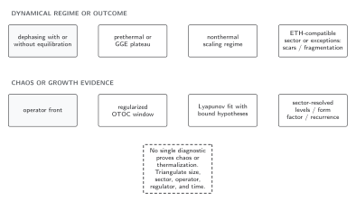
Equilibration is an approach to a stationary value, whereas thermalization additionally requires agreement with the appropriate equilibrium ensemble for a declared observable class. The displayed regimes are arrow-free alternatives, and the separate lower row contains chaos diagnostics rather than necessary stages in one evolution.

Equivalently in prose: test equilibration through time dependence and fluctuations, test thermalization through ensemble predictions and conserved charges, and test chaos separately through operator or spectral observables. Hydrodynamization and pressure isotropy are still different criteria.

Exercises

For $p_n=1/N$, compute the effective dimension and the global Hilbert–Schmidt distance from the diagonal ensemble.

Solution

$d_{\mathrm{eff}}=(N\cdot N^{-2})^{-1}=N$, and the squared distance is $1-1/N$. It approaches one even while the temporal variance of a few-body observable can vanish with $N$.

Suppose a density correlator is described by diffusion after time $t_h$, but its one-particle distribution is visibly anisotropic until $t_i>t_h$. What has been established for $t_h<t<t_i$?

Solution

The measured long-wavelength density mode has hydrodynamized within the stated error. Isotropization of the distribution has not occurred, and full thermalization has not been established.

Continue from relaxation to mechanism

Prethermalization and generalized ensembles explain long-lived nonthermal plateaus. ETH supplies a matrix-element criterion for thermal values. Concrete quench protocols and material realizations continue in Volume XII.

References

• Linden, Noah, Sandu Popescu, Anthony J. Short, and Andreas Winter. “Quantum Mechanical Evolution towards Thermal Equilibrium.” Physical Review E 79 (2009): 061103. doi:10.1103/PhysRevE.79.061103. Open preprint.
• Reimann, Peter. “Foundation of Statistical Mechanics under Experimentally Realistic Conditions.” Physical Review Letters 101 (2008): 190403. doi:10.1103/PhysRevLett.101.190403. Open preprint.
• Short, Anthony J. “Equilibration of Quantum Systems and Subsystems.” New Journal of Physics 13 (2011): 053009. doi:10.1088/1367-2630/13/5/053009. Open preprint.