Nonperturbative Renormalization Schemes and Step Scaling

A renormalization condition need not be evaluated in a loop expansion. It can be imposed directly on regulated correlation functions, provided the condition fixes a closed operator sector and admits a controlled continuum limit. Step scaling then replaces one impossible separation of scales by a chain of finite scale changes, each measured nonperturbatively and extrapolated before the matrices are multiplied.

This page constructs that chain for composite operators. It fixes the direction of every renormalization and evolution matrix, distinguishes finite-volume schemes from off-shell momentum-subtraction schemes, derives composition and finite-scheme covariance, and states the evidence and uncertainty record needed to connect a low scale to a perturbative conversion scale. It defines no current numerical renormalization constants and does not own lattice ensemble generation.

Required background. Operator Anomalous-Dimension Matrices fixes the chapter convention $O_0=ZO$ and $\mathcal D O=-\gamma O$.

Helpful background. Symmetry-Protected Operators, Currents, and Improvement explains when a Ward identity can replace a generic normalization condition and which finite symmetry-restoration terms may remain.

A finite renormalization condition without a loop expansion

Let $O_{\rm lat}$ be a column of bare operators in a regulator with short-distance scale $a$. Introduce a finite intermediate scheme $X$ by

$$\boxed{ O_{\rm R}^{X}(\mu) = \mathcal Z^{X}(g_0,a\mu)\,O_{\rm lat}. }$$

The calligraphic matrix maps bare to renormalized. It is the inverse of the chapter’s bare-from-renormalized matrix:

$$O_{\rm lat} = Z^{X}O_{\rm R}^{X}, \qquad Z^{X}=(\mathcal Z^{X})^{-1}.$$

Keeping these symbols distinct prevents a common reversal in step-scaling ratios.

Choose a matrix of regulated correlation functions

$$F_{j\alpha}(g_0,a\mu,m_{\rm R},\mathcal K)$$

with one insertion of $O_{{\rm lat},j}$. The label $\alpha$ denotes external states, boundary sources, or projectors, and $\mathcal K$ denotes the kinematic and geometric data. External-field or boundary-source normalization factors are understood to have been divided out. A square, nonsingular condition can be written as

$$\left. \mathcal Z^X_{ij}F_{j\alpha} \right|_{ m_{\rm R}=0,\, \mathcal K=\mathcal K_X(\mu) } = F^{\rm tree}_{i\alpha}.$$

Equivalently,

$$\mathcal Z^X = F^{\rm tree}F^{-1}.$$

This equation is a definition, not a perturbative approximation. A numerical path integral may determine $F$ at strong coupling. The scheme is nevertheless fully conventional: it depends on the operator basis, projectors, external states, gauge if one is fixed, boundary conditions, mass prescription, and tree-level normalization.

A valid condition must satisfy more than invertibility at one cutoff:

• the declared operator sector must be closed under all regulator-allowed mixing;
• power-divergent lower-dimensional admixtures must be subtracted rather than hidden in an unstable inverse;
• the same condition must be implementable at several cutoff resolutions;
• symmetry-restoration conditions must be imposed where the regulator breaks a required identity; and
• the resulting step ratios must have a regulator-independent continuum limit.

If more conditions than unknown matrix entries are imposed, the fitting metric and covariance become part of the scheme definition. If $F$ is nearly singular, the corresponding operator directions are not cleanly resolved; a plausible-looking inverse is not evidence of a usable scheme.

Momentum subtraction and finite volume

Two families of intermediate schemes solve different parts of the scale-separation problem.

Off-shell RI/MOM-type conditions

In a regularization-independent momentum-subtraction scheme, amputated off-shell Green functions are evaluated in a fixed gauge and projected at a specified Euclidean momentum configuration. Schematically,

$$\left. \mathcal Z^X_{ij}Z_\Phi^{-n/2} P_\alpha\Gamma_j(p_1,\ldots,p_n) \right|_{ \mathcal K_X(\mu),\,m_{\rm R}=0 } = F^{\rm tree}_{i\alpha}.$$

The gauge, wave-function prescription $Z_\Phi$, projectors $P_\alpha$, momentum routing, and exceptional or nonexceptional kinematics are part of $X$. The original Rome–Southampton construction makes this definition and its generalization to mixing explicit Martinelli et al. 1995, § 2, pp. 84–87.

In a large box, one seeks the window

$$\frac1L \ll \Lambda_{\rm IR} \ll \mu \ll \frac{\pi}{a}.$$

The lower inequality suppresses finite-volume and long-distance contamination; $\Lambda_{\rm IR}\ll\mu$ suppresses condensate and Goldstone-pole effects and improves continuum perturbation theory; $\mu\ll\pi/a$ suppresses discretization artifacts. Exceptional momentum routing can amplify infrared poles, so symmetric nonexceptional RI/SMOM conditions are often preferable when the operator permits them. Gauge-fixing ambiguities, hypercubic artifacts, chiral extrapolation, and projector conditioning remain explicit systematics.

Finite-volume conditions

A finite-volume scheme instead sets

$$\mu=\frac1L$$

and treats the geometry and boundary conditions as part of the renormalization prescription. Ratios of bulk and boundary correlation functions can cancel boundary-field normalizations and can be gauge invariant. The finite volume is not an unwanted effect to be removed: it is the device that defines the scale.

The advantage is recursive scale separation. A single matched pair need only satisfy $a\ll L$; weak-coupling perturbation theory is required only at the high-energy end where conversion to a conventional continuum scheme is performed. Sint gives the finite-volume requirements, matched-lattice construction, operator ratios, and universality test in one framework Sint 2001, §§ 4.1 and 4.4–4.6, pp. 83–86.

Feature	RI/MOM or RI/SMOM	Finite-volume scheme
Scale	External virtuality $\mu$	Inverse size $1/L$
External data	Gauge-fixed off-shell legs and projectors	Boundary or finite-volume correlation functions
Main strength	Direct continuum conversion factors and flexible operator projectors	Recursive running across a large scale range
Main tension	Simultaneously require small infrared and cutoff effects	Boundary artifacts and repeated line-of-constant-physics tuning
Essential check	Momentum-window stability and kinematic variants	Separate continuum limit and step composition
Conversion	Usually perturbative at the chosen $\mu$	Perturbative only after the chain reaches a high scale

The two ideas can also be combined: one may define a finite-volume momentum-subtraction scheme and step its scale. What matters is that all geometry and kinematics remain fixed in dimensionless units while $a/L\to0$.

Matrix step scaling from matched volumes

Fix a scale factor $s>1$ and a mass-independent finite-volume coupling

$$u=\bar g_X^2(L).$$

For a chosen resolution $N=L/a$, tune the bare parameters so that

$$\bar g_X^2(L)=u, \qquad m_{\rm R}=0.$$

At those same bare parameters, evaluate the operator normalization on the paired lattices $L/a=N$ and $sL/a=sN$. Define

$$\begin{aligned} \Sigma_O^X\left(u,\frac aL;s\right) ={}& \mathcal Z^X(g_0,sL/a) \left[ \mathcal Z^X(g_0,L/a) \right]^{-1} \\ &\bigg|_{\bar g_X^2(L)=u,\,m_{\rm R}=0}. \end{aligned}$$

The finite-cutoff matrix depends on the regulator and on $a/L$. Its continuum limit is the operator step-scaling matrix

$$\boxed{ S_O^X(u;s) = \lim_{a/L\to0} \Sigma_O^X\left(u,\frac aL;s\right). }$$

Because the same bare operator column occurs at both volumes,

$$\begin{aligned} O_{\rm R}^X\left(\frac1{sL}\right) &= \mathcal Z^X(sL)\,O_{\rm lat} \\ &= S_O^X(u;s) O_{\rm R}^X\left(\frac1L\right). \end{aligned}$$

Thus the convention on this page runs operators from $\mu=1/L$ down to $\mu/s$. With $\mathcal D O=-\gamma O$,

$$S_O^X(u;s) = \mathcal P \exp\!\left[ -\int_{\ln\mu}^{\ln(\mu/s)} dt\,\gamma^X(t) \right].$$

For a constant anomalous-dimension matrix,

$$S_O^X(u;s)=e^{\gamma^X\ln s}.$$

The sign is therefore fixed: increasing $L$ by $s$ produces $+\gamma\ln s$ in the exponent. The coefficient vector runs in the dual representation,

$$C^X\left(\frac{\mu}{s}\right) = \left[S_O^X(u;s)\right]^{-\mathsf T} C^X(\mu),$$

so $C^{\mathsf T}O$ is unchanged.

The figure should be read from left to right. First inspect where the continuum limit occurs; then follow the matrix product in the middle row. The earlier step acts on the operator column first and therefore appears on the right.

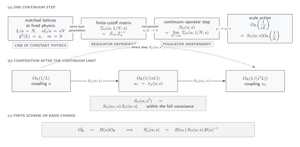
At fixed $u=\bar g^2(L)$ and vanishing renormalized mass, matched resolutions $N$ and $sN$ determine a regulator-dependent ratio $\Sigma_O$. Its $a/L\to0$ limit defines $S_O(u;s)$, which may then be composed and compared with a direct larger step. A finite, coupling-dependent operator-scheme change acts with $B(u)$ and $B(u_1)$ at different endpoints. The original diagram is schematic and not to scale.

The same content in semantic form is:

Stage	Held fixed	Output	Invalid shortcut
Matched pair	$u$, zero-mass condition, action, boundary data, operator projectors	$\Sigma_O(u,a/L;s)$	Comparing unmatched bare parameters
Continuum extrapolation	Physical finite-volume scheme	$S_O(u;s)$	Treating one fine lattice as the continuum
Composition	Coupling sequence and matrix orientation	$S_O(u;s_1s_2)$	Multiplying finite-$a$ matrices from incompatible resolutions
Scheme change	Basis maps at both endpoint couplings	$S'_O=B(u_1)S_OB(u)^{-1}$	Ordinary similarity transformation with one $B$ when $B$ runs

Composition and the low-to-high chain

Let the coupling step be

$$u_1=\sigma_g^X(u;s_1).$$

The exact continuum composition law is

$$\boxed{ S_O^X(u;s_1s_2) = S_O^X(u_1;s_2) S_O^X(u;s_1). }$$

The $s_1$ matrix acts first and sits on the right. This is the discrete counterpart of path ordering. For a direct measurement of the larger step, define the closure residual

$$\Delta_{\rm comp} = S_{O,{\rm direct}}^X(u;s_1s_2) - S_O^X(u_1;s_2)S_O^X(u;s_1).$$

Every entry should be consistent with zero under the joint covariance of the direct and factored determinations. Entrywise error bars are not enough when the same ensembles, tuning interpolations, or normalization matrices occur in both sides.

To climb from a low scale $\mu_0=1/L_0$ to

$$\mu_k=s^k\mu_0, \qquad L_k=\frac{L_0}{s^k},$$

the downward convention is inverted at each stage:

$$\begin{aligned} O_{\rm R}^X(\mu_n) ={}& \left[S_O^X(u_n;s)\right]^{-1} \cdots \left[S_O^X(u_1;s)\right]^{-1} O_{\rm R}^X(\mu_0), \end{aligned}$$

where $u_k=\bar g_X^2(L_k)$. Reversing this product runs along a different RG path when the matrices do not commute.

Exact matrix benchmark

At a fixed point, take the synthetic anomalous-dimension matrix

$$\gamma_\star = \begin{pmatrix} 0&1\\ 0&0 \end{pmatrix}, \qquad \gamma_\star^2=0.$$

For a downward factor-two step,

$$S_O(2) = e^{\gamma_\star\ln2} = \begin{pmatrix} 1&\ln2\\ 0&1 \end{pmatrix}.$$

The direct factor-four result is

$$\begin{aligned} S_O(4) &= e^{\gamma_\star\ln4} \\ &= \begin{pmatrix} 1&2\ln2\\ 0&1 \end{pmatrix} = S_O(2)S_O(2). \end{aligned}$$

The coefficient step is

$$S_C(2) = S_O(2)^{-\mathsf T} = \begin{pmatrix} 1&0\\ -\ln2&1 \end{pmatrix}.$$

This exact, nontrivial mixing example supplies a static benchmark for any step-composition calculation. It tests the factor-two/factor-four relation and the inverse transpose without requiring numerical data.

Finite scheme changes and high-scale conversion

Let two continuum operator schemes be related by a finite matrix

$$O_{\rm R}^{Y}(\mu) = B(g(\mu))O_{\rm R}^{X}(\mu).$$

At the two endpoints, $g(\mu)$ and $g(\mu/s)$ differ. Substitution into the step equation gives

$$\boxed{ S_O^{Y}(u;s) = B(u_1)\, S_O^{X}(u;s)\, B(u)^{-1}. }$$

Only a scale-independent $B$ makes this an ordinary similarity transformation. If the coupling scheme also changes, $u$ and $u_1$ must first be translated to the corresponding endpoint couplings. Coefficients transform as $C^Y=B^{-\mathsf T}C^X$, preserving the complete interaction.

After the nonperturbative chain reaches a scale $\mu_{\rm pt}$ at which a continuum expansion is demonstrably controlled, convert to a target scheme such as $\overline{\rm MS}$:

$$O_{\rm R}^{\overline{\rm MS}}(\mu_{\rm pt}) = R_{X\to\overline{\rm MS}}(\mu_{\rm pt}) O_{\rm R}^{X}(\mu_{\rm pt}).$$

The corresponding Wilson coefficients obey

$$C^{\overline{\rm MS}} = R_{X\to\overline{\rm MS}}^{-\mathsf T}C^X.$$

The intermediate normalization and running can be nonperturbative even though $R_{X\to\overline{\rm MS}}$ is computed perturbatively. Its truncation uncertainty must be kept separate from the continuum extrapolation of $S_O$. Varying perturbative order, conversion scale, and admissible intermediate scheme probes different parts of that error; agreement cannot be assumed.

A current matrix-valued lattice application uses precisely the continuum ratio $\lim_{a\to0}\mathcal Z(\mu_2,a)\mathcal Z(\mu_1,a)^{-1}$ to move four-quark operators to a higher conversion scale and compares direct and subdivided steps Boyle et al. 2024, § IV.B, pp. 034501-8–034501-9. A broader RI′-(S)MOM implementation shows how cutoff artifacts grow at high $\mu$ while perturbative conversion errors grow at low $\mu$, and treats their separation through continuum ratios and analysis variants Bali et al. 2021, §§ VII–IX, pp. 094511-12–094511-17.

If the chain crosses a particle threshold, an EFT matching matrix and a change in the running theory are required. That operation belongs to Matching, Decoupling, and Threshold Evolution; it is not another step in a fixed theory.

Continuum-limit evidence for every step

A credible determination follows this order.

1. Freeze the scheme. State the action, boundary conditions, coupling definition, mass condition, operator basis, projectors or boundary sources, external-field factors, gauge, kinematics, and tree normalization.

2. Close the regulator-level sector. Include all mixing allowed by the regulator. Determine power-divergent and symmetry-restoration subtractions before asking for a logarithmic step matrix.

3. Tune a line of constant physics. For each resolution $N$, tune the bare parameters to the same $u$ and zero-mass condition. Record interpolation residuals and their covariance.

4. Measure matched pairs. At one tuned bare point, evaluate both $N$ and $sN$. Preserve correlations between the two normalization matrices.

5. Diagnose the matrix inverse. Report singular values or condition numbers, symmetry-forbidden entries, projector redundancy, and stability under admissible condition changes.

6. Extrapolate each step. Use several $a/L$ values and a Symanzik-motivated form such as

   $$\Sigma_O\left(u,\frac aL;s\right) = S_O(u;s) + A_1\left(\frac aL\right)^p + A_2\left(\frac aL\right)^{p+1} +\cdots .$$

   The leading power $p$ follows from the action, operator, boundaries, and improvement program; it is not automatically two. Fit matrix entries jointly where their covariance is available, vary the fit range and admissible correction terms, and show that the conclusion does not depend on one coarse resolution.

7. Test universality and composition. Compare regulators, discretizations, or improvement choices when available, and compare a direct larger step with the product of separately extrapolated steps.

8. Convert only in an overlap regime. Demonstrate perturbative stability at $\mu_{\rm pt}$ and propagate the conversion matrix with the same operator orientation.

The individual $\mathcal Z$ matrices may diverge as $a\to0$; their ratio at two physical scales can still have a finite continuum limit. This is why the extrapolated step matrix, rather than a plateau in a bare renormalization factor, is the primary running observable.

Uncertainty and covariance record

The final result is a correlated matrix product. Its uncertainty record should expose the following sources rather than collapse them prematurely into one percentage.

Source	Diagnostic or variation	Required propagation
Sampling and autocorrelation	Binned histories, integrated autocorrelation, topological-sector checks	Joint resampling of all correlators, volumes, and matrix entries
Coupling and mass tuning	Alternative interpolation forms; residual offsets in $u$ and $m_{\rm R}$	Derivatives or repeated resampling through the tuning fit
Finite-volume scheme realization	Boundary contamination, aspect-ratio and source-placement checks	Treat deviations from the declared geometry as errors; do not “remove” the defining $L$
Cutoff extrapolation	Resolution cuts, justified powers, improvement variants, regulator comparison	Correlated continuum fit for every step
Sector closure and power subtraction	Enlarged bases, subtraction conditions, symmetry-forbidden entries	Propagate the full mixing and subtraction covariance
Projector or boundary-source conditioning	Singular values, alternate complete projectors, tree-level normalization checks	Retain correlations introduced by the common inverse
Gauge and kinematics	Gauge-fixing tolerance, copy study where relevant, exceptional versus nonexceptional momenta	Keep scheme variants distinct until converted
Scale setting	Alternative reference scales and their correlations	Shift every dimensional endpoint coherently
Step composition	Direct $s_1s_2$ result versus factored product	Use the covariance of the closure residual
Perturbative conversion	Order, scale, and intermediate-scheme variations	Separate conversion truncation from nonperturbative running
Threshold matching	Matching-scale and truncation variations	Correlate with running on both sides of the threshold

Products of correlated random matrices are generally non-Gaussian. A joint bootstrap, jackknife, or posterior draw through tuning, inversion, continuum fits, composition, and conversion is safer than adding entrywise percentages in quadrature. Report uncertainties on physical coefficient–operator combinations as well as on basis-dependent matrix entries.

What the construction establishes

Nonperturbative normalization does not mean scheme-independent normalization. It means that the defining Green functions and the scale-changing ratios were evaluated without expanding them in a weak coupling. The continuum scheme, operator basis, and finite normalization remain choices.

Step scaling also does not create a continuum limit from one lattice spacing. Each step needs its own matched sequence of resolutions. Nor does reaching a numerically high scale prove perturbation theory is adequate there; conversion stability must be demonstrated.

This page supplies the continuum definitions, matrix checks, and evidence design. Nonperturbative Renormalization, Mixing, and Step Scaling develops ensemble construction, continuum inference for actual data, and production determinations.

Common pitfalls

Reversing the ratio. With $O_{\rm R}=\mathcal ZO_{\rm lat}$, the step from $1/L$ to $1/(sL)$ is $\mathcal Z(sL)\mathcal Z(L)^{-1}$. The reverse ratio runs in the opposite direction.

Composing before extrapolating. A product of finite-cutoff matrices can combine different artifacts and tuning errors. Extrapolate the declared steps, retain their covariance, and then test continuum composition.

Treating every finite-volume dependence as an error. Dependence on the prescribed $L$, aspect ratio, and boundary conditions defines the scheme. Only failure to realize that prescription is a systematic deviation.

Ignoring matrix conditioning. A small statistical error on correlators can become a large, biased error after an ill-conditioned inversion. Report the resolved directions and test alternate complete projectors.

Calling the final answer fully nonperturbative after a low-scale conversion. If the target-scheme conversion is truncated perturbation theory, its uncertainty remains even when all preceding steps were nonperturbative.

Exercises

1. Derive the ratio direction

Assume

$$O_{\rm R}(1/L)=\mathcal Z(L)O_{\rm lat}, \qquad O_{\rm R}(1/(sL))=\mathcal Z(sL)O_{\rm lat}.$$

Derive the matrix that maps the first renormalized operator to the second, and translate it to the convention $O_{\rm lat}=ZO_{\rm R}$.

Solution

Eliminate the bare column:

$$O_{\rm lat} = \mathcal Z(L)^{-1}O_{\rm R}(1/L).$$

Therefore

$$O_{\rm R}(1/(sL)) = \mathcal Z(sL)\mathcal Z(L)^{-1} O_{\rm R}(1/L).$$

Since $Z=\mathcal Z^{-1}$, the same matrix is

$$S_O = Z(sL)^{-1}Z(L).$$

Writing $Z(sL)Z(L)^{-1}$ would mix the two conventions and reverse the map.

2. Prove composition and scheme covariance

Let $u_1=\sigma_g(u;s_1)$ and let $O^Y=B(u)O^X$. Derive the two-step composition law and the transformation of a one-step matrix.

Solution

Successive operator equations give

$$\begin{aligned} O^X(\mu/(s_1s_2)) &= S_O^X(u_1;s_2)O^X(\mu/s_1) \\ &= S_O^X(u_1;s_2)S_O^X(u;s_1)O^X(\mu). \end{aligned}$$

Hence

$$S_O^X(u;s_1s_2) = S_O^X(u_1;s_2)S_O^X(u;s_1).$$

For the scheme change,

$$\begin{aligned} O^Y(\mu/s) &= B(u_1)O^X(\mu/s) \\ &= B(u_1)S_O^X(u;s)B(u)^{-1}O^Y(\mu). \end{aligned}$$

Therefore

$$S_O^Y(u;s) = B(u_1)S_O^X(u;s)B(u)^{-1}.$$

Different endpoint matrices are required when $B$ depends on the running coupling.

3. Check the dual nilpotent step

For

$$S_O(2) = \begin{pmatrix} 1&\ell\\ 0&1 \end{pmatrix}, \qquad \ell=\ln2,$$

compute $S_O(2)^2$ and $S_O(2)^{-\mathsf T}$. Verify the coefficient–operator pairing after one step.

Solution

Direct multiplication gives

$$S_O(2)^2 = \begin{pmatrix} 1&2\ell\\ 0&1 \end{pmatrix} = S_O(4).$$

The inverse and inverse transpose are

$$S_O(2)^{-1} = \begin{pmatrix} 1&-\ell\\ 0&1 \end{pmatrix}, \qquad S_O(2)^{-\mathsf T} = \begin{pmatrix} 1&0\\ -\ell&1 \end{pmatrix}.$$

If $O'=S_OO$ and $C'=S_O^{-\mathsf T}C$, then

$$C'^{\mathsf T}O' = C^{\mathsf T}S_O^{-1}S_OO = C^{\mathsf T}O.$$

Continue

• Continue to Scale Independence and the Callan–Symanzik Equation to connect discrete steps with continuous RG equations.
• Continue to Matching, Decoupling, and Threshold Evolution when the scale chain changes its active theory.
• Use Nonperturbative Renormalization, Mixing, and Step Scaling for the production lattice workflow.
• Return to the Composite Operators and Mixing overview for the complete source-to-coefficient chain.

References

• Bali, G. S., S. Bürger, S. Collins, M. Göckeler, M. Gruber, S. Piemonte, A. Schäfer, A. Sternbeck, and P. Wein. 2021. “Nonperturbative Renormalization in Lattice QCD with Three Flavors of Clover Fermions: Using Periodic and Open Boundary Conditions.” Physical Review D 103: 094511. DOI. Open PDF.
• Boyle, Peter A., Felix Erben, Jonathan M. Flynn, Nicolas Garron, James Kettle, Rajnandini Mukherjee, and Julian T. Tsang. 2024. “Kaon Mixing beyond the Standard Model with Physical Masses.” Physical Review D 110: 034501. DOI. Open PDF.
• Martinelli, Guido, C. Pittori, Christopher T. Sachrajda, Massimo Testa, and Anastassios Vladikas. 1995. “A General Method for Non-Perturbative Renormalization of Lattice Operators.” Nuclear Physics B 445: 81–105. DOI. Open PDF.
• Sint, Stefan. 2001. “Non-Perturbative Renormalization in Lattice Field Theory.” Nuclear Physics B — Proceedings Supplements 94: 79–94. DOI. Open PDF.