Tree-Level Matching and Classical Elimination

Tree-level matching replaces virtual heavy exchange by local interactions whose coefficients reproduce low-energy amplitudes. Solving the heavy field’s classical equation does this because substituting the stationary solution generates every tree graph with internal heavy lines. The replacement is local only after expanding the heavy inverse operator in momenta and light masses over the heavy scale. This page carries that procedure through dimension eight and checks the first omitted power directly against the full amplitude.

Required background. Integrating Out Heavy Fields supplies the exact nonlocal Wilson action and its boundary-condition dependence. The Action Principle and Field Equations supplies stationary variation and integration by parts. Helpful background. Local versus Integrated Operator Redundancies distinguishes an action-level equation-of-motion relation from a local operator identity.

Why the classical solution generates heavy-exchange trees

Let $\phi$ denote all light fields and $H$ all fields to be removed. A heavy classical configuration $H_c[\phi]$ obeys

$$\left. \frac{\delta S[\phi,H]}{\delta H} \right|_{H=H_c[\phi]} =0$$

with the boundary condition appropriate to the matching object. The tree-level light action is

$$S_{\mathrm{EFT}}^{(0)}[\phi] = S[\phi,H_c[\phi]].$$

This statement is not merely a saddle-point mnemonic. Differentiating the stationarity condition gives

$$\frac{\delta H_c}{\delta\phi} = -\left(S_{HH}^{(2)}\right)^{-1}S_{H\phi}^{(2)},$$

where the derivatives on the right are evaluated at $H_c$. A second light-field derivative therefore contains

$$S_{\mathrm{EFT},\phi\phi}^{(2)} = S_{\phi\phi}^{(2)} -S_{\phi H}^{(2)} \left(S_{HH}^{(2)}\right)^{-1} S_{H\phi}^{(2)}.$$

The inverse heavy Hessian is precisely the internal heavy propagator, while the adjacent derivatives are its endpoint vertices. Further differentiation branches this structure into all tree topologies containing heavy internal lines. Loops do not appear: they require the fluctuation determinant or higher terms in the quantum saddle expansion. Henning, Lu, and Murayama formulate tree matching as evaluating the ultraviolet Lagrangian at its heavy-field solution in Henning, Lu, and Murayama 2016, § 1, pp. 2–5 and § 2, pp. 9–17, PDF.

The exact inverse $\left(S_{HH}^{(2)}\right)^{-1}$ is generally nonlocal. Thus classical elimination and the local EFT expansion are two separate operations, as panel (a) emphasizes. Panel (b) anticipates the additional full-minus-EFT subtraction required once loops are included.

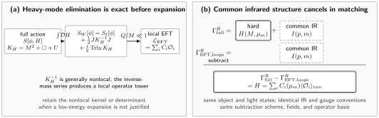
Heavy-field elimination and matching separate two steps. Panel (a) integrates a Gaussian heavy field with quadratic operator $K_H=M^2+\Box+U[\phi]$ and light source $J[\phi]$, producing an exact, generally nonlocal source term and a field-dependent determinant; only for $Q/M\ll1$ are these expanded into local operators. Panel (b) shows a renormalized loop matching condition: with the matching object, light states, infrared prescription, gauge, scheme, fields, and basis aligned, the common infrared term cancels and the remainder fixes the hard Wilson coefficients. The diagram is schematic and not to scale.

Iterative elimination of a heavy scalar

Consider in four spacetime dimensions

$$\mathcal L = \frac12(\partial\phi)^2 +\frac12(\partial H)^2 -\frac12M^2H^2 -\frac g2H\phi^2,$$

where $[\phi]=[H]=1$ and $[g]=1$. After integrating the heavy kinetic term by parts, define

$$K_H=M^2+\Box, \qquad J=\frac g2\phi^2, \qquad \mathcal L_H=-\frac12HK_HH-JH.$$

The heavy equation and its low-derivative solution are

$$K_HH_c=-J,$$ $$\begin{aligned} H_c &=-\frac g2\frac1{M^2+\Box}\phi^2\\ &=-\frac{g}{2M^2}\phi^2 +\frac{g}{2M^4}\Box\phi^2 -\frac{g}{2M^6}\Box^2\phi^2 +O(M^{-8}). \end{aligned}$$

This is also an iterative calculation: insert the leading algebraic solution into the derivative term, improve it by two derivatives, and repeat until the target inverse-mass order is reached. Substitution into both the quadratic and linear heavy terms is essential. At the stationary point,

$$-\frac12H_cK_HH_c-JH_c = +\frac12JK_H^{-1}J,$$

so the local tree Lagrangian becomes

$$\begin{aligned} \mathcal L_{\mathrm{EFT}}^{(0)} =\mathcal L_\ell &+\frac{g^2}{8M^2}\phi^4 -\frac{g^2}{8M^4}\phi^2\Box\phi^2\\ &+\frac{g^2}{8M^6}\phi^2\Box^2\phi^2 +O(M^{-8}). \end{aligned}$$

The three displayed interactions have canonical dimensions four, six, and eight. The alternating signs in the action follow from expanding $(M^2+\Box)^{-1}$; on a momentum eigenstate, $\Box$ contributes $-q^2$, turning their amplitude contributions into positive powers of $q^2/M^2$ below the heavy pole.

For a nonlinear heavy sector, write $H_c=H^{(0)}+H^{(1)}+\cdots$ in the chosen counting and solve the equation order by order. Each correction must be substituted into the complete action, including interactions quadratic and higher in $H$. Keeping only the source term or only the leading heavy solution generally loses tree topologies or produces a wrong symmetry factor.

Amplitude matching through dimension eight

Take four external light momenta incoming and define

$$s=(p_1+p_2)^2, \qquad t=(p_1+p_3)^2, \qquad u=(p_1+p_4)^2.$$

Strip the common overall factor $i$ from the scattering amplitude. The full theory gives one heavy exchange in each pairing,

$$\mathcal A_{\mathrm{full}} = g^2\left( \frac1{M^2-s} +\frac1{M^2-t} +\frac1{M^2-u} \right).$$

The compact interaction $g^2\phi^2F(\Box)\phi^2/8$ has eight assignments of the four identical external fields for each unordered pairing. Its factor $1/8$ therefore leaves unit weight for each of the $s$, $t$, and $u$ channels. Expanding $F$ through $\Box^2$ gives

$$\mathcal A_{\mathrm{EFT}}^{(d\leq8)} = g^2\left[ \frac3{M^2} +\frac{s+t+u}{M^4} +\frac{s^2+t^2+u^2}{M^6} \right].$$

At leading order the same combinatorics can be read as

$$4!\left(\frac{g^2}{8M^2}\right) = \frac{3g^2}{M^2},$$

which is the sum of three leading exchange terms. The exact remainder after the dimension-eight truncation is

$$\Delta\mathcal A = \mathcal A_{\mathrm{full}} -\mathcal A_{\mathrm{EFT}}^{(d\leq8)} = g^2\sum_{x=s,t,u} \frac{x^3}{M^6(M^2-x)}.$$

If $|s|,|t|,|u|\leq\rho M^2$ with $\rho<1$, then

$$|\Delta\mathcal A| \leq \frac{g^2}{M^2} \frac{1}{1-\rho} \sum_{x=s,t,u}\left|\frac{x}{M^2}\right|^3.$$

This establishes an absolute $O(g^2Q^6/M^8)$ remainder, or a relative $O((Q/M)^6)$ error against the leading amplitude, within the geometric expansion’s domain. The bound is conditional: closeness to the heavy pole, a new threshold, or an accidentally suppressed retained amplitude can make it uninformative.

Here is a direct numerical check at physical massless kinematics. Set

$$\frac{(s,t,u)}{M^2} = z(0.09,-0.04,-0.05), \qquad F\equiv\frac{M^2\mathcal A}{g^2}.$$

The relation $s+t+u=0$ holds, and changing $z$ scales every invariant while fixing the scattering angle.

$z$	$\max\lvert x\rvert/M^2$	$F_{\mathrm{full}}$	$F_{d\leq8}$	$F_{\mathrm{full}}-F_{d\leq8}$	Residual divided by $z^3$
0.25	0.0225	3.000771234	3.000762500	$8.7337\times10^{-6}$	$5.5896\times10^{-4}$
0.50	0.0450	3.003122332	3.003050000	$7.2332\times10^{-5}$	$5.7865\times10^{-4}$
1.00	0.0900	3.012820513	3.012200000	$6.2051\times10^{-4}$	$6.2051\times10^{-4}$

The nearly constant last column displays the predicted $z^3$, hence $Q^6$, onset; its mild drift is the sum of still higher powers. A reproducible calculation can vary the hierarchy and retained order. Burgess develops the same logic—nonlocal exchange, inverse-mass expansion, and observable comparison—in Burgess 2021, §§ 2.2–2.3, pp. 26–38.

For massless on-shell scattering the dimension-six amplitude term vanishes because $s+t+u=0$. This cancellation does not set its action coefficient to zero. The operator contributes for off-shell legs, nonzero light masses, background fields, and other processes, so an on-shell match must contain enough independent data to determine every coefficient combination claimed.

Normalization, basis changes, and matching records

Three choices should be recorded before comparing coefficients.

• Field normalization. Canonical kinetic terms and unit LSZ residues must refer to the same light-field coordinates on both sides. A finite field redefinition moves coefficients even when the S-matrix is unchanged.
• Operator normalization. Writing $C\phi^4$, $C\phi^4/4!$, or $C(\phi^2)^2$ assigns different numerical values to the symbol $C$. Derive the vertex once rather than inferring its factor by inspection.
• Expansion and basis. Expand the same invariants to the same order before applying integration by parts or equations of motion. For example,

$$-\phi^2\Box\phi^2 \simeq (\partial_\mu\phi^2)(\partial^\mu\phi^2) =4\phi^2(\partial\phi)^2,$$

where $\simeq$ denotes equality in the integrated action after discarding the declared boundary term. Subsequent use of the light equation of motion can trade this interaction for mass and self-interaction operators. It is not a pointwise identity and can generate contact terms in local correlators.

A robust workflow is therefore: eliminate the heavy field in a convenient generating basis; expand to a declared order; reproduce a spanning set of low-energy amplitudes or Green functions; map to the reduced basis; and repeat at least one observable check. Coefficients are basis coordinates, whereas the matching prediction is invariant under a complete, consistently truncated basis transformation.

Domain and failure conditions

Classical elimination reproduces the desired tree coefficients when the heavy equation has the relevant perturbative solution, its inverse carries the matching observable’s boundary condition, all retained kinematics lie inside the analytic low-energy domain, and the local operator set is complete through the target order. The method must be amended when any of the following occurs:

• a heavy pole or multiparticle threshold lies in the kinematic domain;
• the heavy Hessian develops a zero mode or the background changes which fields are heavy;
• gauge constraints, ghosts, or multiple saddles are omitted from the elimination;
• a loop-sized coefficient is requested, since determinants, counterterms, mixed heavy–light loops, and EFT subtraction then enter; or
• a reduced basis is imposed before the off-shell or contact terms needed to complete the match have been tracked.

Classical elimination also does not remove light propagation. Tree graphs made only from light internal lines are computed in the EFT from its retained dynamics; they are not Wilson coefficients. At loop level, this shared low-energy physics is precisely what must cancel between the two theories before the hard coefficient is isolated.

Common pitfalls

Substituting only into the interaction. The heavy kinetic and mass terms contribute at the same order as the source interaction. Substitution into the complete stationary action produces the factor $1/2$ and the correct sign.

Matching a coefficient before fixing normalization. Identical physics can appear as $C\phi^4$ or $C'\phi^4/4!$. Compare vertices or amplitudes after declaring field and operator normalization.

Reading a kinematic zero as a redundant operator. The $s+t+u$ term vanishes for massless on-shell four-point scattering, but not for arbitrary matching data. Redundancy requires a valid action-level transformation with its sources, contact terms, boundaries, and truncation order tracked.

Using the derivative series at the pole. The local series is an expansion around small invariants and cannot reproduce the heavy resonance with finitely many terms. Near $s=M^2$, retain the heavy degree of freedom or use a description designed for the resonant region.

Exercises

Derive the exact remainder for one channel after retaining $1/M^2+x/M^4+x^2/M^6$, and prove the stated three-channel bound.

Solution

For $r=x/M^2$,

$$\frac1{M^2-x} = \frac1{M^2}(1+r+r^2) +\frac1{M^2}\frac{r^3}{1-r}.$$

The last term is $x^3/[M^6(M^2-x)]$. If $|r|\leq\rho<1$, its magnitude is at most $|r|^3/[M^2(1-\rho)]$. Summing the triangle inequality over $s,t,u$ gives the bound.

Show that integrating the dimension-six term by parts gives the coefficient $g^2/(2M^4)$ multiplying $\phi^2(\partial\phi)^2$.

Solution

With the boundary term discarded,

$$\int d^4x\,\phi^2\Box\phi^2 = -\int d^4x\,(\partial_\mu\phi^2)(\partial^\mu\phi^2).$$

Since $\partial_\mu\phi^2=2\phi\partial_\mu\phi$, the term

$$-\frac{g^2}{8M^4}\phi^2\Box\phi^2$$

is action-equivalent to $g^2\phi^2(\partial\phi)^2/(2M^4)$ under the declared boundary condition.

References

• Burgess, C. P. Introduction to Effective Field Theory: Thinking Effectively about Hierarchies of Scale. Cambridge: Cambridge University Press, 2021. DOI
• Henning, Brian, Xiaochuan Lu, and Hitoshi Murayama. “One-Loop Matching and Running with Covariant Derivative Expansion.” Journal of High Energy Physics 2018, no. 1 (2018): 123. DOI; arXiv