Universality Classes and Scaling Functions

Microscopically different systems belong to the same universality class when their long-distance trajectories approach the same fixed point through the same physical scaling directions. They can then share critical exponents, normalized scaling functions, and amplitude ratios even though their critical temperatures, coupling coordinates, lattice spacings, and individual amplitudes differ. A convincing universality test must remove these nonuniversal metric factors without giving the collapse enough freedom to become automatic.

Required background. Critical Surfaces, Crossover, and Corrections to Scaling explains basins, tuning, and irrelevant corrections. Helpful background. Symmetry Realization and Order Parameters clarifies which symmetry and order-parameter data are actually being compared.

What defines a universality class

A fixed point and its basin provide the RG definition. Microscopic actions $S_A$ and $S_B$ can differ by many couplings, but if their relevant scaling fields are matched and their remaining difference lies in irrelevant directions, then coarse graining suppresses that difference:

$$S_A(k)-S_B(k) = \sum_a c_a \left(\frac{k}{\Lambda}\right)^{\omega_a} \mathcal O_a+cdots, \qquad \omega_a>0.$$

The leading fixed-point data survive, while the coefficients $c_a$ determine nonuniversal corrections and the rate of approach.

Dimension and a familiar symmetry label are not, by themselves, a complete specification. A static universality claim should declare at least:

Defining datum	Why it matters
Dimension and spacetime or spatial interpretation	Changes canonical dimensions, phase space, and the available fixed points
Long-distance degrees of freedom and order-parameter representation	Determines which operators and defects can become relevant
Internal, spacetime, discrete, gauge, and anomaly constraints	Restricts the action and operator mixing; the representation matters as well as the group name
Locality or interaction range	Long-range kernels can be relevant and lead to a different fixed point
Tuned relevant fields and basin	Selects the critical endpoint rather than a first-order region or another fixed point
Geometry and boundary condition for finite-size or boundary observables	Changes otherwise universal finite-size and surface scaling functions
Quenched disorder or other additional slow structure	Can introduce new relevant perturbations and a new class

Dynamic universality requires more information: conserved quantities, reversible couplings, noise, and kinetic coefficients can change the dynamical exponent while leaving the static fixed point unchanged. Those data belong to Dynamic Universality Classes.

Matching one or two numerical exponents is therefore evidence, not a definition. Distinct fixed points can have close exponents, and an apparent match over a finite window can arise from crossover. Agreement of several operator dimensions, normalized scaling functions, amplitude ratios, symmetry sectors, and correction exponents is much harder to fake. Wilson and Kogut explain the RG origin of this loss of microscopic information in Wilson and Kogut 1974, §§ 11–12, pp. 152–176.

Metric factors and universal functions

For a model labeled $i$, let $\tau_i$ and $h_i$ be convenient raw coordinates near its critical point. They need not already be normalized scaling fields. Introduce nonuniversal metric factors

$$\widetilde\tau_i=a_{t,i}\tau_i, \qquad \widetilde h_i=a_{h,i}h_i.$$

The singular equation of state can be written

$$M_i(\tau_i,h_i) = m_{0,i}|\widetilde\tau_i|^{\beta_{\mathrm{mag}}} \mathcal M_\pm(z_i), \qquad z_i = \frac{\widetilde h_i} {|\widetilde\tau_i|^{\beta_{\mathrm{mag}}\delta}}.$$

The exponents and the function $\mathcal M_\pm$ are universal after its normalization is fixed. The three displayed constants are coordinate and amplitude conventions. They are not all independent under stronger two-scale-factor universality assumptions, but retaining them here makes the normalization choices explicit.

A convenient collapse plot uses

$$Y_i \equiv \frac{M_i} {m_{0,i}|\widetilde\tau_i|^{\beta_{\mathrm{mag}}}}, \qquad Y_i=\mathcal M_\pm(z_i).$$

Changing $a_{t,i}$ or $a_{h,i}$ stretches the axes; changing $m_{0,i}$ stretches the ordinate. A universal function becomes a falsifiable object only after these freedoms are fixed by stated normalization conditions, such as one susceptibility amplitude and one coexistence-curve amplitude, rather than tuned point by point.

The large- and small-argument limits encode named exponents. In the symmetric phase,

$$\mathcal M_+(z)\sim z \quad(z\to0), \qquad \mathcal M_+(z)\sim z^{1/\delta} \quad(z\to\infty).$$

The first limit gives $M\sim h|\tau|^{-\gamma}$ because $\gamma=\beta_{\mathrm{mag}}(\delta-1)$; the second gives the critical isotherm $M\sim h^{1/\delta}$. A proposed function that fails either limit is not merely poorly normalized—it is inconsistent with the exponent definitions.

Worked collapse of two scalar models

Take a synthetic benchmark with

$$\beta_{\mathrm{mag}}=\frac13, \qquad \delta=5, \qquad \mathcal M_+(z) =z(1+z^2)^{-2/5}.$$

The function has the required limits $\mathcal M_+(z)\sim z$ at small $z$ and $\mathcal M_+(z)\sim z^{1/5}$ at large $z$. Define two microscopic scalar models with different metric data:

$$\begin{array}{c|ccc} &a_t&a_h&m_0\\ \hline A&1&1&2\\ B&4&1/2&5 \end{array}$$

Choose $\widetilde\tau_A=\widetilde\tau_B=10^{-2}$. The raw temperature coordinates are therefore $\tau_A=10^{-2}$ and $\tau_B=2.5\times10^{-3}$. Sampling three common scaled fields gives:

$z$	$h_A$	$M_A$	$h_B$	$M_B$	$Y_A=Y_B$
$0.25$	$1.1604\times10^{-4}$	$0.10514$	$2.3208\times10^{-4}$	$0.26285$	$0.24401$
$1$	$4.6416\times10^{-4}$	$0.32655$	$9.2832\times10^{-4}$	$0.81638$	$0.75786$
$4$	$1.8566\times10^{-3}$	$0.55494$	$3.7133\times10^{-3}$	$1.38734$	$1.28789$

The raw fields and magnetizations do not coincide. After the declared transformations,

$$z_A=z_B=z, \qquad \frac{M_A}{2|\widetilde\tau_A|^{1/3}} = \frac{M_B}{5|\widetilde\tau_B|^{1/3}} = \mathcal M_+(z).$$

This exact collapse is a calculation from the supplied function, not empirical evidence for a real universality class. It demonstrates what the test removes. For measured models the leading form is instead

$$Y_i(z,\widetilde\tau_i,L_i) = \mathcal M_+(z) +c_i|\widetilde\tau_i|^{\omega\nu} \mathcal M_{1,+}(z) +d_iL_i^{-\omega} \mathcal M_{L,+}(z) +\cdots.$$

The correction amplitudes $c_i$ and $d_i$ can differ in sign and size. A credible collapse extrapolates them or varies the proximity and size windows; it does not absorb them into a separate axis rescaling for every dataset.

Universal amplitudes and invariant combinations

Individual amplitudes depend on the normalization of $\tau$, $h$, the field, and the unit of length. Ratios can cancel those metric factors. Familiar examples include

$$\frac{\xi_+}{\xi_-}, \qquad \frac{\Gamma_+}{\Gamma_-}, \qquad R_\xi^+ =\xi_+\left(\alpha A_+\right)^{1/d},$$

in a common thermodynamic normalization, with the $\alpha\to0$ case treated by its appropriate limiting or logarithmic definition. The definitions, phases, and hyperscaling assumptions needed for the last combination must be fixed. Boundary conditions and geometry must be specified for finite-size amplitudes. A ratio formed from inconsistent definitions is not made universal by being dimensionless.

Normalized scaling functions contain more information than a small exponent list. The equation of state, finite-size free energy, two-point momentum dependence, and crossover functions probe different projections of the fixed-point theory. Their normalizations should be stated close to the result because a change of metric factors can make two equivalent universal functions look different.

Widom’s homogeneous equation of state supplies the scaling-function structure in Widom 1965, pp. 3898–3905. Privman and Fisher show how universal finite-size functions and amplitude combinations retain explicit geometry and boundary-condition dependence in Privman and Fisher 1984, pp. 322–327.

Scaling windows and falsifiable collapse

For each microscopic model, a static scaling window should satisfy competing inequalities. In schematic form,

$$a_i\ll\xi_i\ll L_i, \qquad |u_{a,i}|\,\xi_i^{-\omega_a}\ll1,$$

while every unintended relevant field remains small on the scale $\xi_i$. Finite-size scaling deliberately studies $\xi_i/L_i=O(1)$ instead, but then $L_i$ becomes a scaling variable rather than an ignored correction.

A robust collapse protocol is:

1. Fix critical coordinates and metric factors from declared observables, with covariance and uncertainty.
2. Hold those normalizations fixed for other observables and for a withheld portion of the data.
3. Vary the minimum correlation length, maximum $\xi/L$, and correction ansatz.
4. Compare the residuals with statistical and systematic errors rather than judging a plot by eye.
5. Test asymptotic limits, amplitude ratios, and at least one correction exponent.
6. Repeat across microscopic actions whose leading irrelevant amplitudes differ.

If a collapse requires a high-order warp of each axis, separate critical points for each field value, or a different exponent in every window, it is describing the data rather than testing universality.

Boundaries and emergent symmetry

Universality has precise failure modes. A long-range tail can become relevant; quenched disorder can destabilize a clean fixed point; a cubic or lattice anisotropy can remain relevant; topological defects can supply missing degrees of freedom; and a first-order transition has no diverging correlation length on which the fixed-point argument can act. Harris gives a classic relevance test for weak random-mass disorder in Harris 1974, pp. 1671–1692, but its hypotheses must be checked before applying the inequality.

Emergent symmetry is stronger than approximate rotational appearance or matching leading exponents. At the putative symmetric fixed point, every allowed symmetry-breaking perturbation must be irrelevant or tuned, and observables should organize into the predicted symmetry multiplets. A small negative anisotropy exponent can produce an exceptionally long crossover, so finite systems may look symmetric before ultimately departing.

The shared phase portrait summarizes the mechanism: irrelevant microscopic differences shrink along the critical surface, while any unmatched relevant component eventually separates the flows.

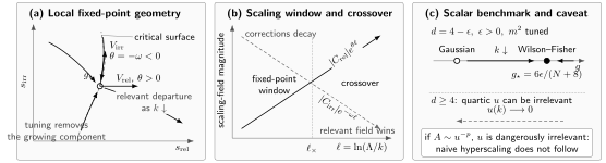
A fixed point organizes local flow, not every global trajectory. Panel (a) shows the critical surface tangent to the irrelevant eigendirection and the relevant departure under infrared flow. Panel (b) compares $e^{\theta\ell}$ growth with $e^{-\omega\ell}$ corrections for $\ell=\ln(\Lambda/k)$. Panel (c) shows the tuned one-loop $O(N)$ scalar trajectory from the Gaussian point to $g_\star=6\epsilon/(N+8)$ and the dangerously irrelevant-coupling exception to naive hyperscaling. The diagram is schematic and not to scale.

Fixed-point evidence matrix

A universality claim is strongest when methods with different assumptions converge on compatible invariant data. The table keeps the evidence routes distinct; read each row as a statement of what is controlled, what is observed, and where the inference stops.

Evidence route	Essential assumptions and control	Direct outputs or observables	Dominant systematics and evidence ceiling
Perturbative expansion	A small $\epsilon$, weak fixed-point coupling, large-$N$ parameter, or other declared expansion; specified renormalization scheme and operator sector	Beta-function zeros, stability eigenvalues, anomalous dimensions, and resummed exponent or amplitude-ratio estimates	Missing orders, asymptotic-series resummation, scheme and operator truncation; controlled local evidence within the expansion domain, not a global existence proof at order-one parameters
Lattice finite-size scaling	A Euclidean discretization in the target basin; controlled critical, continuum, and infinite-volume limits; reflection positivity when used	Correlation lengths, step scaling, Binder-type ratios, spectra, exponents, amplitude ratios, and scaling functions	Cutoff and volume extrapolation, critical tuning, autocorrelation, action dependence, and analytic continuation; strong nonperturbative IR evidence for the simulated universality class
Functional RG	An exact flow equation combined with a declared ansatz, projection, regulator, identity constraints, and convergence tests	Global flow portraits, effective potentials, fixed-point spectra, equations of state, and crossover trajectories	Truncation, projection, regulator dependence, symmetry identities, convexity, and numerics; quantitative candidate evidence unless convergence is independently controlled
Conformal bootstrap	Conformal invariance, crossing, a symmetry sector, unitarity or reflection positivity when imposed, and explicit gap assumptions	Allowed or excluded regions for operator dimensions and OPE coefficients; islands and universal CFT data	Derivative and spin truncations, assumed gaps, navigator or optimization choices, and numerical certification; characterizes or excludes a CFT under stated assumptions but does not supply an RG trajectory
Rigorous or constructive analysis	A precise lattice or continuum model, norm, positivity domain, and theorem hypotheses, often in restricted dimensions or coupling ranges	Existence or nonexistence, controlled continuum correlations, bounds, and in some cases complete RG trajectories	Transfer is limited by theorem hypotheses and model class; strongest conclusion inside the proved domain, with no automatic extension to nearby physical theories

Representative primary analyses illustrate the distinct ceilings: the epsilon expansion constructs a perturbative fixed point Wilson and Fisher 1972, pp. 240–243; finite-size lattice scaling controls volume and correction terms Hasenbusch 2010, §§ II–V; effective-average-action studies expose truncation and regulator choices Berges, Tetradis, and Wetterich 2002, §§ 2–3, pp. 245–287; bootstrap bounds assume crossing and unitarity El-Showk et al. 2012, §§ II–IV; and rigorous construction can establish a complete trajectory for a precisely defined modified model Abdesselam 2007, pp. 727–772.

The Gaussian and Wilson–Fisher Fixed Points page next calculates a controlled fixed point whose basin supplies the chapter’s scalar benchmark.

Common pitfalls

Equating symmetry and dimension with a complete class label. Interaction range, field representation, relevant defects, disorder, and boundary data can change the fixed point. Dynamic questions also require conserved modes and kinetics.

Optimizing the collapse by eye. Enough independent offsets, stretches, and window choices can align almost any smooth datasets. Metric factors and exclusions need declared determination rules and uncertainty propagation.

Calling every dimensionless ratio universal. Universality requires cancellation of all metric factors and identical definitions, geometry, and boundary conditions. A dimensionless bare coupling is usually scheme dependent.

Inferring emergent symmetry from leading exponents alone. The symmetry-breaking eigenoperators and multiplet structure must also agree, especially when anisotropy is only weakly irrelevant.

Exercises

1. Check the synthetic scaling limits

For $\mathcal M_+(z)=z(1+z^2)^{-2/5}$, derive its small- and large-$z$ limits and verify that the latter corresponds to $\delta=5$.

Solution

For $z\ll1$, $(1+z^2)^{-2/5}=1+O(z^2)$, so $\mathcal M_+(z)=z+O(z^3)$. For $z\gg1$,

$$\mathcal M_+(z) \sim z(z^2)^{-2/5} =z^{1/5}.$$

The critical-isotherm limit is therefore $M\sim h^{1/5}$, which means $\delta=5$.

2. Undo the metric factors

For model $B$ in the worked example, use $\tau_B=2.5\times10^{-3}$, $h_B=9.2832\times10^{-4}$, and $M_B=0.81638$. Recover $z$ and $Y$.

Solution

The normalized fields are

$$\widetilde\tau_B=4\tau_B=10^{-2}, \qquad \widetilde h_B=\frac12h_B=4.6416\times10^{-4}.$$

Since $|\widetilde\tau_B|^{\beta\delta}=(10^{-2})^{5/3}=4.6416\times10^{-4}$, one obtains $z=1$. Also

$$Y =\frac{0.81638}{5(10^{-2})^{1/3}} \simeq0.75786,$$

which equals $2^{-2/5}=\mathcal M_+(1)$ within rounding.

3. Separate a correction from a metric factor

Two models obey $Y_i(z,\tau)=\mathcal M(z)+c_i|\tau|^{0.5}\mathcal M_1(z)$. Explain how measurements at four decreasing $|\tau|$ values can distinguish this from a constant ordinate rescaling.

Solution

A metric factor multiplies the ordinate by the same constant at every proximity to criticality. The correction changes with $|\tau|^{0.5}$ and extrapolates linearly in that variable at fixed $z$. Fit the four values at each $z$ to a common intercept and model-dependent slopes $c_i\mathcal M_1(z)$. Stability of the intercept under removal of the largest $|\tau|$ point supports the correction interpretation; a persistent constant offset instead signals a normalization mismatch.

4. Test an emergent-symmetry claim

A lattice model has leading exponents compatible with an $O(N)$ fixed point, but the leading allowed anisotropy has $\theta_{\mathrm{aniso}}=0.03$. Does the model generically display $O(N)$ symmetry asymptotically in the IR?

Solution

No. In the chapter convention, positive $\theta_{\mathrm{aniso}}$ is relevant and grows under infrared coarse graining. The anisotropy must be forbidden or tuned for the trajectory to remain on the $O(N)$ critical surface. Because the exponent is small, finite systems can show a long approximately symmetric crossover before the departure becomes visible.

References

• Abdesselam, Abdelmalek. “A Complete Renormalization Group Trajectory Between Two Fixed Points.” Communications in Mathematical Physics 276 (2007): 727–772. DOI. Open PDF.
• Berges, Jürgen, Nikolaos Tetradis, and Christof Wetterich. “Non-Perturbative Renormalization Flow in Quantum Field Theory and Statistical Physics.” Physics Reports 363 (2002): 223–386. DOI. Open PDF.
• El-Showk, Sheer, Miguel F. Paulos, David Poland, Slava Rychkov, David Simmons-Duffin, and Alessandro Vichi. “Solving the 3D Ising Model with the Conformal Bootstrap.” Physical Review D 86 (2012): 025022. DOI. Open PDF.
• Harris, A. Brooks. “Effect of Random Defects on the Critical Behaviour of Ising Models.” Journal of Physics C: Solid State Physics 7 (1974): 1671–1692. DOI.
• Hasenbusch, Martin. “Finite Size Scaling Study of Lattice Models in the Three-Dimensional Ising Universality Class.” Physical Review B 82 (2010): 174433. DOI. Open PDF.
• Privman, Vladimir, and Michael E. Fisher. “Universal Critical Amplitudes in Finite-Size Scaling.” Physical Review B 30 (1984): 322–327. DOI.
• Widom, Benjamin. “Equation of State in the Neighborhood of the Critical Point.” Journal of Chemical Physics 43 (1965): 3898–3905. DOI.
• Wilson, Kenneth G., and Michael E. Fisher. “Critical Exponents in 3.99 Dimensions.” Physical Review Letters 28 (1972): 240–243. DOI.
• Wilson, Kenneth G., and John Kogut. “The Renormalization Group and the $\epsilon$ Expansion.” Physics Reports 12 (1974): 75–200. DOI.