Scale Separation, Locality, and the Domain of an EFT

A hierarchy of scales makes a local effective field theory possible only when the omitted dynamics responds analytically to the low external momenta in the domain being studied. The nearest pole, threshold, cut, or other nonanalyticity limits that expansion. This page derives locality from the heavy-field response, distinguishes analytic domain from numerical breakdown, and gives a practical test for deciding whether a state may be removed.

Required background. Effective Field Theory as a Controlled Expansion defines the EFT control statement and heavy-mediator benchmark. Poles, Cuts, Thresholds, and Stable Particles explains how propagating states and multiparticle thresholds appear as amplitude singularities. Helpful background. Analyticity and Crossing of Amplitudes develops the channel-dependent analytic structure used here.

Locality from analytic short-distance response

Split the fields into light variables $\phi$ and a heavy variable $H$. Eliminating $H$ exactly gives a functional of $\phi$ that is generally nonlocal. A local EFT exists when that functional can be expanded in derivatives over the momenta of interest.

For the scalar model

$$\mathcal L_H = -\frac12H(\Box+M^2)H -\frac g2H\phi^2,$$

the classical equation is

$$(\Box+M^2)H_{\mathrm{cl}} = -\frac g2\phi^2.$$

Solving and substituting back gives the exact tree-level contribution

$$\Delta\mathcal L_{\mathrm{nonlocal}} = \frac{g^2}{8} \phi^2\frac{1}{M^2+\Box}\phi^2.$$

The inverse differential operator connects separated spacetime points, so this is not yet a local Lagrangian. When derivatives acting on the light fields satisfy $|\Box|\ll M^2$, expand

$$\frac{1}{M^2+\Box} = \frac1{M^2} \left( 1-\frac{\Box}{M^2} +\frac{\Box^2}{M^4} -\cdots \right).$$

Thus

$$\Delta\mathcal L_{\mathrm{local}} = \frac{g^2}{8M^2}\phi^4 -\frac{g^2}{8M^4}\phi^2\Box\phi^2 +\frac{g^2}{8M^6}\phi^2\Box^2\phi^2 +\cdots.$$

For a momentum $q$ entering the heavy line, $\Box\to-q^2$, so the alternating derivative series reproduces

$$\frac{1}{M^2-q^2} = \frac1{M^2} \sum_{n=0}^{\infty} \left(\frac{q^2}{M^2}\right)^n.$$

Locality is therefore an expansion statement. The full theory remains local, the exact light-only functional is nonlocal, and the low-energy derivative expansion restores locality order by order within its analytic domain. Burgess derives the low-energy action from the separation of high- and low-energy states in Burgess 2021, §§ 1.2 and 2.2–2.3, pp. 9–16 and 26–39.

Singularities set the analytic radius

Let a full-theory amplitude $F(z)$ depend on a complexified invariant $z$ and be analytic around an expansion point $z_0$. Cauchy’s formula gives

$$F(z) = \sum_{n=0}^{\infty} \frac{F^{(n)}(z_0)}{n!}(z-z_0)^n$$

inside the largest disk centered on $z_0$ that contains no singularity. The coefficients are local Wilson coefficients or combinations of them; the radius is the distance to the nearest pole, branch point, or other obstruction in the complex plane.

Several consequences follow.

1. A large mass ratio is not enough. One must know which singularity is nearest in each channel and for the chosen external quantum numbers.
2. A crossed-channel pole can constrain an expansion even when the physical $s$-channel energy is below its first production threshold.
3. A multiparticle cut can be nearer than a single-particle pole, or a symmetry can remove the residue of a nominally nearby state from a particular amplitude.
4. Expanding around a different kinematic point changes the relevant analytic distance and the convenient operator organization.

For the heavy-mediator amplitude, the three geometric series require

$$|s|<M^2, \qquad |t|<M^2, \qquad |u|<M^2.$$

At the chapter’s fixed angle, $|s|$ is the largest invariant, so $E/M<1$ is the mathematical convergence condition for the tree-level series. A precision calculation normally imposes a stronger condition because $E/M=0.9$ is inside the disk but does not give a rapidly convergent truncation.

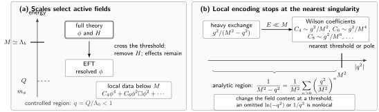
This is the relationship summarized in the shared scale/content map. Inspect the separation between the physical threshold and the smaller working scale $Q$, and the distinction between an active light field and its forbidden replacement by a local coefficient.

Scale separation determines content and locality. Below the schematic threshold $M\simeq\Lambda_b$, the resolved field $\phi$ remains active while the heavy field $H$ is encoded by coefficients $C_4,C_6,C_8,\ldots$ ordered in $q=Q/\Lambda_b$. The geometric propagator expansion is local only for $|q^2|<M^2$; crossing the threshold or omitting a massless nonanalytic contribution requires different degrees of freedom. The diagram is schematic and not to scale.

Four boundaries that should not be collapsed

The word “cutoff” is often asked to carry several incompatible meanings. A careful EFT calculation separates at least four boundaries.

Boundary	Definition	How it is determined
Analyticity boundary	Nearest singularity to the expansion point in the relevant complex kinematic variable	Spectrum, thresholds, crossing, and Landau singularities
EFT breakdown scale $\Lambda_b$	Scale where the chosen fields or counting cease to provide systematic control	Known omitted states plus residual and coefficient diagnostics
Working upper limit $Q_{\max}$	Largest scale actually admitted in a fit or prediction	Target accuracy and validation data; normally $Q_{\max}<\Lambda_b$
Regulator scale $\Lambda_{\mathrm{reg}}$	Auxiliary parameter defining loop integrals or a regulated Hamiltonian	Chosen calculation scheme; predictions must be regulator independent to the claimed order

In a simple weakly coupled heavy exchange, the analyticity boundary and $M$ can provide a good estimate of $\Lambda_b$. They need not be identical in general. A broad resonance, a strongly coupled continuum, an anomalously low collective mode, a finite-density surface, or an enhanced coefficient can make practical breakdown occur earlier. Conversely, a state at mass $M$ that does not couple in the sector being studied need not set the first correction for that observable.

The renormalization scale $\mu$ is different again. It redistributes logarithms between Wilson coefficients and matrix elements. Moving $\mu$ within a sensible range does not cross a physical threshold unless the EFT content is explicitly changed and a matching condition is applied.

Light nonanalyticities must remain dynamical

Suppose a loop of a massless retained field contributes

$$F_{\mathrm{light}}(s) \supset \alpha\ln\frac{-s-i0}{\mu^2}.$$

No Taylor series around $s=0$ can represent the branch point there. A Wilson coefficient obtained by removing that light field would have to be nonlocal, defeating the proposed local EFT. The correct split keeps the light field active: its loop matrix element reproduces the logarithm, while the coefficient contains only contributions analytic at low momentum apart from its renormalization-scale dependence.

The same reasoning applies to:

• a nearly on-shell particle whose propagator denominator is comparable to the residual momentum;
• a Goldstone boson, photon, or other gapless excitation;
• a Fermi surface or hydrodynamic mode that produces low-energy nonanalytic response; and
• a shallow bound state whose pole lies parametrically below the nominal hard scale.

Sometimes one introduces an auxiliary field to make a recurring pole explicit. That is not adding ultraviolet information; it is choosing degrees of freedom that render the resolved analytic structure local and the counting transparent.

Thresholds change more than coefficients

Below a stable heavy-particle production threshold, virtual heavy effects can be expanded locally. At or above the threshold, the heavy state can propagate over long times, and the amplitude develops the associated imaginary part or cut. A theory without that state cannot reproduce unitarity by adjusting real local coefficients alone.

Crossing a threshold can therefore change:

• the active fields and asymptotic states;
• the beta functions and anomalous dimensions;
• the operator basis and its symmetry realization;
• the number and type of kinematic regions; and
• the counting of widths, residual momenta, or velocities.

The transition is handled by matching two EFTs in an overlap region, followed by separate running on either side. Running and Matching across Multiple Thresholds develops that ladder. If a resonance is narrow and the observable probes its pole region, the appropriate description may retain a resonant field with a complex pole rather than jump directly from the full theory to a contact expansion.

Convergent, asymptotic, and practically useful expansions

Three questions should be asked separately.

Does the Taylor series converge? For a single heavy propagator, yes, inside the disk bounded by its pole. The exact radius follows from analytic structure.

Does the complete EFT expansion converge? Not necessarily. Perturbative loop coefficients can grow factorially, several expansions can be nested, and the derivative series can be only asymptotic after other contributions are included. A controlled asymptotic expansion remains useful when it has a window in which successive terms decrease and the remainder is estimated near the chosen truncation.

Is the truncated prediction accurate enough? Even a convergent series may converge too slowly for a desired tolerance. If the first omitted relative correction is estimated as $c_{k+1}q^{k+1}$, the target $\delta$ requires

$$|c_{k+1}|q^{k+1}\lesssim\delta.$$

For coefficients of order one, a ten-percent expansion parameter can support far greater precision at order $q^4$ than a fifty-percent parameter. The working domain is therefore accuracy dependent.

A domain declaration in practice

Before using a local EFT, record:

1. Kinematics: the range of every independent invariant, light mass, background gradient, and multiplicity.
2. Resolved singularities: all poles, cuts, pinch surfaces, and collective modes inside or near that range.
3. Active fields: one field or mode for each long-distance propagation mechanism the EFT must reproduce.
4. Hard scales: the nearest omitted structures and the evidence used to estimate $\Lambda_b$.
5. Expansion variables: $Q/\Lambda_b$ and any additional ratios, with rules for mixed terms.
6. Validation window: observables or energies withheld from coefficient determination and used to test the predicted residual.
7. Validity limit: a threshold, residual-scaling failure, coefficient instability, or target-accuracy condition that ends extrapolation.

This declaration is stronger than listing masses. It connects the spectrum to the analytic structure, the analytic structure to the fields, and the fields to a falsifiable expansion.

Common pitfalls

A mass gap proves locality for every observable. The gap must separate the states that couple in the chosen channel, and no other light singularity may be present. Backgrounds, boundaries, or nearly on-shell configurations can introduce additional low scales.

Inside the convergence radius means safely inside the EFT domain. Mathematical convergence does not guarantee rapid convergence at the retained order. The working domain must meet the requested accuracy and pass residual tests.

A loop logarithm can always be placed in a Wilson coefficient. Hard logarithms can be part of matching coefficients, but nonanalytic dependence generated by retained light modes belongs to EFT matrix elements. The full-minus-effective separation is developed in Infrared Cancellation, Regulators, and Matching Consistency.

One breakdown scale controls every channel. A common conservative $\Lambda_b$ can be useful, but selection rules and different nearest singularities can produce channel-dependent convergence. State the choice rather than silently using the most favorable scale.

Exercises

The function $F(s)=1/(M^2-s)+a/(4M^2-s)$ is expanded around $s=0$, with $a\neq0$. What is the radius of convergence, and what changes if a symmetry sets the residue of the first pole to zero?

Solution

For nonzero residues at both poles, the nearest singularity is at $s=M^2$, so the Taylor series has radius $M^2$. If the first residue vanishes exactly, the $s=M^2$ pole is absent from this amplitude and the nearest singularity moves to $s=4M^2$. The spectrum alone does not determine the radius; the state must couple in the sector and observable under consideration.

A truncated observable has relative remainder $r\simeq2q^4$. Find the largest $q$ compatible with a one-percent target under this estimate.

Solution

Require $2q^4\leq0.01$. Hence

$$q\leq\left(\frac{0.01}{2}\right)^{1/4}\simeq0.266.$$

This is a practical working limit inferred from the target accuracy, even if the analytic series converges for all $q<1$.

References

• Burgess, C. P. Introduction to Effective Field Theory: Thinking Effectively about Hierarchies of Scale. Cambridge: Cambridge University Press, 2021. DOI
• Weinberg, Steven. “Phenomenological Lagrangians.” Physica A: Statistical Mechanics and its Applications 96 (1979): 327–340. DOI