

Basis Translation, Scheme Dependence, and Reproducibility
A basis translation is reliable only when it maps the operators, the dual Wilson coefficients, the renormalization prescription, and the perturbative truncation together. A matrix of operator names is not enough: its orientation, normalization, flavor ordering, scale, evanescent definitions, input parameters, and finite scheme terms determine what the numbers mean.
This page fixes those data explicitly. It first translates a two-dimensional scalar quotient and checks both a four-point amplitude and an RG trajectory. It then extends the linear map to coupling-dependent schemes and nonlinear EFT redefinitions, ending with a machine-readable record that can be regenerated and tested.
Required background. Local Field Redefinitions and the Equivalence Theorem supplies the order-by-order action map. Wilson-Coefficient Evolution supplies the dual RG equation for coefficient columns.
Helpful background. Anomalous Dimensions and Wilson-Coefficient Evolution fixes the operator-mixing convention. Scheme Transformations and RG Invariants explains coupling-scheme changes. Fierz Relations and Dimension-Specific Identities, Evanescent Operators, and On-Shell Amplitude Bases supply the algebraic and physical checks used below.
Operator and coefficient maps
Section titled “Operator and coefficient maps”Write each ordered operator basis as a column. For two bases describing the same physical quotient, define the operator map by
where rows label the target basis and columns label the source basis . If the effective interaction is
then the coefficient column transforms contragrediently:
The transpose is forced by the invariant pairing ; it is not a convention that may be chosen independently. The inverse maps are
These formulae require to be invertible on the declared physical quotient. A rectangular candidate-to-basis reduction matrix can be useful, but it is not an invertible basis translation until redundant directions have been removed or a common quotient and its projectors have been specified.
Operator normalization belongs inside . Thus a change from to , a sign change, a conjugate-completed flavor convention, or a permutation of indices is part of the matrix rather than prose attached afterward. Wilson-coefficient exchange formats implement the same principle by coupling coefficient data to a named EFT, a named basis, a renormalization scale, and real or complex value conventions Aebischer et al. 2018, § 2, preprint pp. 3–5, Open PDF.
First application: two scalar bases at dimension eight
Section titled “First application: two scalar bases at dimension eight”Consider a real massless scalar in four dimensions with a symmetry and free EOM . Work through order and define monomials without factorial normalizations. The dimension-eight quotient has the two independent representatives
Choose a second, deliberately non-orthogonal basis
Exact arithmetic gives
Therefore
Substitution verifies the full interaction, not merely the matrices:
The four-particle contact amplitude supplies an independent physical check. About the vacuum , has no four-point vertex, whereas the convention established on the preceding page gives
It follows that
This amplitude tests the derivative coordinate and the coefficient transpose. It cannot detect the independent eight-field coordinate , so it does not replace the exact two-coordinate round trip. A complete certification combines algebraic invertibility with observables sensitive to the sectors needed for the intended application.
Anomalous dimensions under a moving basis
Section titled “Anomalous dimensions under a moving basis”Let denote the full RG derivative, including beta functions acting on any couplings inside the basis map, and choose
Differentiating gives
Only a scale-independent produces a pure similarity transformation. The endpoint form is often safer in code. If transports operator columns and transports coefficient columns from to , then
An exact algebraic fixture checks all orientations. It is not a loop calculation for the scalar theory. Take constant above and
Then
For and an initial coefficient , the source-basis solution is
Alternatively, translate first:
Mapping the endpoint back with reproduces the source-basis solution exactly. This trajectory check catches a misplaced transpose, an incorrectly ordered endpoint matrix, or a sign error in the anomalous-dimension convention.
Finite schemes, evanescent operators, and input choices
Section titled “Finite schemes, evanescent operators, and input choices”A practical conversion often combines a basis map with a finite renormalization. If changes representatives and changes the finite prescription, define
where is a declared loop-counting coupling. Then
and
For a constant and coupling-independent ,
with . A finite coefficient shift and the corresponding change in are two faces of the same scheme map; applying only one gives spurious scale or scheme dependence.
The counterterm matrix also depends on what is held fixed. With and the same bare column on both sides, implies
If both the bare and renormalized columns are transformed by the same constant , instead . Confusing these two comparisons is a common source of incorrect similarity formulae.
Evanescent definitions generate finite even when the four-dimensional physical representatives look identical. In , a change
multiplies counterterms and leaves a finite physical term. A translation record must therefore name the -dimensional algebra, prescription when relevant, evanescent column and ordering, its physical parts, and the finite projection condition. Herrlich and Nierste derive the resulting physical-sector scheme transformation in Herrlich and Nierste 1995, §§ 2–4, preprint pp. 3–11, Open PDF.
An input-parameter scheme is additional data. For example, two electroweak calculations may use different measured quantities to eliminate the same Lagrangian parameters. EFT corrections then shift those elimination formulae, so the conversion is a finite re-expansion involving Standard Model parameters and Wilson coefficients, not generally a constant operator matrix. State the renormalized inputs, quantities held fixed, scale, parameter definitions, and expansion order; express both results in one input scheme before comparing coefficients or observables.
Nonlinear maps across EFT orders
Section titled “Nonlinear maps across EFT orders”Perturbative field redefinitions make coefficient maps triangular in the EFT expansion rather than purely linear. A representative form through is
where is a convention-dependent bilinear map induced by the lower-order field transformation and by re-expanding the action. The order-consistent inverse is
Dropping the quadratic term while retaining dimension-eight effects compares two different truncations. The same order accounting must include parameter shifts, source terms relevant to the chosen observables, and loop corrections. Criado and Pérez-Victoria derive these higher-order effects and explain why a first-order EOM substitution alone does not define a higher-order field redefinition Criado and Pérez-Victoria 2019, §§ 3 and 5.1, preprint pp. 9–12 and 16–18, Open PDF.
A machine-readable translation record
Section titled “A machine-readable translation record”A portable record needs stable operator definitions, exact matrices, and theory metadata in the same object. WCxf provides a broadly used schema for exchanging Wilson coefficients once an EFT and basis have been defined. AutoEFT demonstrates that explicit contractions and basis data can also be represented in machine-readable form Harlander and Schaaf 2024, § 5.2, preprint pp. 29–33, Open PDF. Neither a basis name nor a coefficient file by itself supplies an unrecorded evanescent prescription, finite input-scheme conversion, or nonlinear truncation rule.
The scalar benchmark can be serialized as follows. Rational entries remain strings so that a parser does not silently replace exact arithmetic by binary floating point.
{ "record_version": "1.0", "scope": { "spacetime_dimension": "4", "metric_signature": "+---", "fields": [{"name": "phi", "reality": "real", "mass": "0"}], "exact_symmetries": ["Z2"], "eom_quotient": "box(phi)=0", "eft_order": "Lambda^-4" }, "source_basis": { "name": "D", "operators": [ {"name": "D1", "definition": "phi^8", "normalization": "no factorial"}, {"name": "D2", "definition": "(d_mu phi d^mu phi)^2", "normalization": "unit monomial"} ] }, "target_basis": { "name": "R", "operators": [ {"name": "R1", "definition": "D1 + D2"}, {"name": "R2", "definition": "D2"} ] }, "operator_map": { "orientation": "R = B D", "B": [["1", "1"], ["0", "1"]], "B_inverse": [["1", "-1"], ["0", "1"]] }, "coefficient_map": { "orientation": "C_R = B^(-T) C_D", "B_inverse_transpose": [["1", "0"], ["-1", "1"]] }, "renormalization": { "regulator": "dimensional regularization, d=4-2 epsilon", "subtraction_scheme": "MSbar", "scale": "mu", "finite_scheme_map": "identity in the displayed tree benchmark", "evanescent_operators": [] }, "truncation": { "eft": "through Lambda^-4", "amplitude": "tree level", "rg": "constant-gamma algebraic fixture, not scalar loop data" }, "checks": { "operator_round_trip": "B_inverse B = identity exactly", "coefficient_round_trip": "B^T B^(-T) = identity exactly", "four_point": "2 (C_R1+C_R2) P/Lambda^4 = 2 C_D2 P/Lambda^4", "P": "s^2+t^2+u^2", "rg_fixture": "B gamma_D B_inverse = diag(1,-1)" }}A production exporter should canonicalize this object, attach a SHA-256 checksum, and retain the tool version, dependency lockfile, source commit or archive hash, and generation command. The checksum certifies bytes, not physics, so it accompanies rather than replaces the algebraic and observable checks.
Acceptance tests and limitations
Section titled “Acceptance tests and limitations”The construction below separates the five checks that a trustworthy translation must pass. Inspect especially the distinction between closure and four-dimensional projection, and between the operator matrix and its dual coefficient matrix.
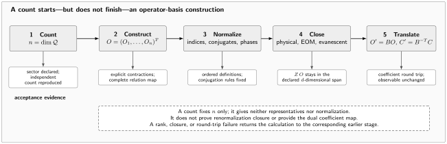
An operator-basis result is a five-stage package. Counting fixes ; construction supplies explicit contractions and relations; normalization fixes ordering, conjugation, and phases; closure enlarges the -dimensional renormalization space when EOM or evanescent operators are required; and translation applies with the dual coefficient map . The lower row states the required checks at each stage. A count alone is neither an explicit basis nor proof of RG closure. The diagram is schematic and not to scale.
At minimum, test the following on the common declared subspace:
- Exact forward and inverse products are identity matrices after all rational and symbolic substitutions.
- Operator and coefficient maps preserve through the stated EFT and loop order.
- At least one amplitude, correlator, decay rate, or other physical benchmark agrees after translating every parameter and matrix element.
- RG evolution commutes with translation, using endpoint matrices when the map runs.
- The target basis is closed under the retained -dimensional counterterms before evanescent projection.
- A clean software rerun reproduces operator ordering, matrix entries, ranks, and checksums.
Numerical agreement alone is weak evidence when a matrix is nearly singular or a relation depends on a tolerance. Retain exact arithmetic where possible; otherwise publish singular values, precision, threshold, conditioning, and a higher-precision stability check. A map may also be valid only on a flavor slice, CP sector, mass limit, or perturbative subspace. Encode that domain rather than padding the matrix with zeros and calling it universal.
One reproducible calculation can test the exact quotient maps, amplitude coordinates, anomalous-dimension similarity fixture, and endpoint evolution formula. It cannot infer missing normalization or scheme metadata from a numerical coefficient vector.
The operator-basis reproducibility record
Section titled “The operator-basis reproducibility record”Use one record for the basis definition, the translation, and its verification. The same fields support a hand calculation, a symbolic notebook, or an exchange file.
| Record | Declare before reduction | Verification retained with the result |
|---|---|---|
| Field content and order | Spacetime dimension, dynamical fields, exact symmetries, charges, EFT grading, and truncation | Every candidate and relation has the declared labels and order |
| Flavor, Hermiticity, and CP | Flavor-index ranges, conjugation rule, coefficient reality conditions, and CP convention | Conjugate completion and independent real parameter count agree |
| Operator definition | Ordered names, explicit index contractions, derivative placement, signs, and normalization factors | Each symbolic or numerical column maps to one unambiguous operator |
| Renormalization data | Regulator, subtraction scheme, gauge convention when relevant, renormalization scale , and coupling definitions | Coefficients and matrix elements use the same scheme and scale |
| Dimensional identities | Dimension used for Lorentz and spinor algebra, prescription when present, and evanescent-operator definitions | The renormalized basis closes before any four-dimensional projection |
| Redundancy generators | IBP currents and boundary conditions, lower-order EOM, field maps, and algebraic identities | Every relation row is reproducible from a displayed generator |
| Basis map | Candidate and reduced dimensions, matrix orientation, exact rank, pivots, and representative ordering | Nullities and ranks satisfy the quotient dimension and no pivot is tolerance-dependent |
| Coefficient map | Dual transformation, transpose convention, finite shifts, and perturbative order | is unchanged through the retained order |
| Implementation identity | Source or notebook version, dependency versions, input hash, and output checksum | A clean rerun reproduces the ordered map and checksum |
| Round trip and physics | Forward and inverse maps on the common subspace plus one amplitude, correlator, or counting benchmark | The round trip is the identity and the benchmark is basis independent to the stated tolerance |
For the scalar record, retain the ordered columns and , the orientation , both exact inverse matrices, the no-factorial normalization, the convention, and the amplitude polynomial . For the RG fixture, state explicitly that is synthetic algebraic test data and retain the sign convention .
Common pitfalls
Section titled “Common pitfalls”Applying the same matrix to operators and coefficients. If , then . Using on both generally changes the interaction and every observable derived from it.
Quoting an anomalous dimension without its basis convention. A coupling-dependent map adds . Even for constant maps, operator and coefficient anomalous dimensions are transposes under the conventions used here.
Calling a four-dimensional Fierz map a dimensional-scheme translation. Four-dimensional identities can remove evanescent directions too early. Close and renormalize the -dimensional space first, then apply the finite physical projection.
Round-tripping beyond the declared truncation. A perturbative inverse is the identity only through the order retained. Products of discarded terms should be marked as higher order, not treated as a failed or exact check.
References
Section titled “References”-
Aebischer, Jason, et al. 2018. “WCxf: An Exchange Format for Wilson Coefficients beyond the Standard Model.” Computer Physics Communications 232: 71–83. DOI. Open PDF.
-
Criado, Juan Carlos, and Manuel Pérez-Victoria. 2019. “Field Redefinitions in Effective Theories at Higher Orders.” Journal of High Energy Physics 2019 (3): 038. DOI. Open PDF.
-
Harlander, Robert V., and Magnus C. Schaaf. 2024. “AutoEFT: Automated Operator Construction for Effective Field Theories.” Computer Physics Communications 300: 109198. DOI. Open PDF.
-
Herrlich, Stefan, and Ulrich Nierste. 1995. “Evanescent Operators, Scheme Dependences and Double Insertions.” Nuclear Physics B 455 (1–2): 39–58. DOI. Open PDF.