Momentum-Shell Integration and Rescaling

A momentum-shell step has two logically separate parts. First integrate fields in a declared band of momenta; then rescale momenta, coordinates, and the remaining field so that the cutoff returns to its original numerical value. For one real scalar with interaction $\lambda\phi^4/4!$ in $d=4-\epsilon$, this procedure gives, in the convention defined below,

$$\frac{dr}{d\ell} = 2r+\frac{u}{2(1+r)}+O(u^2), \qquad \frac{du}{d\ell} = \epsilon u-\frac{3u^2}{2(1+r)^2}+O(u^3).$$

Here $\ell$ increases toward the infrared, $r=m^2/k^2$, and $u=K_d\lambda k^{d-4}$. The canonical and fluctuation terms therefore come with signs appropriate to an infrared-directed flow. The calculation is perturbative, uses a sharp spherical shell, and projects the resulting action onto its mass and quartic coordinates; it is not an exact two-coupling closure.

Required background. Wilsonian Coarse Graining and Theory Space defines the blocking map, the retained field, quasi-locality, and the distinction between a full trajectory and a finite projection.

Helpful background. Gaussian Vectors, Processes, Random Distributions, and Wick Structure supplies the Gaussian cumulants and contractions used in the shell average.

A scalar shell step with declared conventions

At a cutoff $k$, take the Euclidean action

$$\begin{aligned} S_k[\phi] &= S_{0,k}[\phi]+V_k[\phi],\\ S_{0,k}[\phi] &= \frac12 \int_{|p|<k}\frac{d^dp}{(2\pi)^d} \,(p^2+m^2)\phi(p)\phi(-p),\\ V_k[\phi] &= \frac{\lambda}{4!}\int d^dx\,\phi(x)^4. \end{aligned}$$

The kinetic coefficient is one, $m^2$ and $\lambda$ are the dimensionful coordinates before the step, and the $\mathbb Z_2$ symmetry forbids odd powers of $\phi$. Set

$$k'=ke^{-\delta\ell}, \qquad b\equiv\frac{k}{k'}=e^{\delta\ell}, \qquad \delta\ell>0,$$

and split $\phi=\varphi+\chi$ into retained modes $|p|<k'$ and shell modes $k'<|p|<k$. The shell covariance is

$$C_>(q) = \frac{\mathbf 1_{\{k'<|q|<k\}}}{q^2+m^2}.$$

This denominator must not vanish in the shell. The expansion below is most reliable for weak $\lambda$, a thin shell, and external momenta well below $k'$.

The Wilson action before rescaling is defined by

$$e^{-S_{k'}[\varphi]} = e^{-S_{0,k'}[\varphi]} \left\langle e^{-V_k[\varphi+\chi]} \right\rangle_>,$$

where $\langle\cdots\rangle_>$ is the normalized Gaussian average with covariance $C_>$. Wilson and Kogut introduce precisely this sequence—eliminate rapidly varying modes, restore the momentum range, and normalize the field—in Wilson and Kogut 1974, § 3, pp. 99–101.

Cumulants and the induced local action

Taking the logarithm gives the connected-cumulant expansion

$$\begin{aligned} S_{k'}[\varphi] = S_{0,k'}[\varphi] &+\langle V_k\rangle_>\\ &-\frac12 \left( \langle V_k^2\rangle_> -\langle V_k\rangle_>^2 \right) +O(\lambda^3). \end{aligned}$$

Define the shell integrals

$$I_n(k,\delta\ell) \equiv \int_{k'<|q|<k} \frac{d^dq}{(2\pi)^d} \frac{1}{(q^2+m^2)^n}.$$

Wick contraction of the first cumulant yields

$$\langle V_k\rangle_> = \int d^dx \left[ \frac{\lambda}{4!}\varphi^4 +\frac{\lambda I_1}{4}\varphi^2 +\frac{\lambda I_1^2}{8} \right].$$

The three terms are respectively the original quartic interaction, a tadpole mass shift, and a vacuum-energy shift. At second order, the connected contraction with two shell lines between the vertices contains

$$-\frac{\lambda^2}{16} \int d^dx\,d^dy\, \varphi(x)^2 C_>(x-y)^2\varphi(y)^2.$$

For a retained field varying slowly on the scale $k^{-1}$,

$$\int d^dy\,C_>(x-y)^2\varphi(y)^2 = I_2\varphi(x)^2 +\text{terms with derivatives}.$$

Matching the local terms to $\delta m^2\varphi^2/2+\delta\lambda\varphi^4/4!$ gives

$$\boxed{ \delta m^2=\frac{\lambda}{2}I_1+O(\lambda^2), \qquad \delta\lambda=-\frac32\lambda^2 I_2+O(\lambda^3) }.$$

The factor $3/2$ is not an arbitrary beta-function convention: $36$ choices select two shell fields at each quartic vertex, the connected contraction of the two pairs contributes a factor $2$, the cumulant contributes $-1/2$, and matching to $1/4!$ completes the count.

This local projection does not exhaust the shell average. Momentum-dependent four-point terms, derivative operators, higher powers of the field, and vacuum terms are generated according to their symmetry and momentum routing. A sharp boundary also makes an expansion at external momenta comparable with $k'$ nonanalytic. The displayed local expansion is a low-external-momentum statement, not a claim that the complete blocked vertex is a polynomial.

Thin-shell evaluation

Let

$$K_d \equiv \frac{S_{d-1}}{(2\pi)^d} = \frac{2}{(4\pi)^{d/2}\Gamma(d/2)}.$$

Here $S_{d-1}=2\pi^{d/2}/\Gamma(d/2)$ is the area of the unit $(d-1)$-sphere.

Radial integration over a shell of thickness $k\delta\ell+O(\delta\ell^2)$ gives

$$I_n = K_d\frac{k^d}{(k^2+m^2)^n}\,\delta\ell +O(\delta\ell^2).$$

Consequently, before rescaling,

$$\begin{aligned} \delta m^2 &= \frac{\lambda K_d}{2} \frac{k^{d-2}}{1+m^2/k^2}\,\delta\ell +O(\lambda^2,\delta\ell^2),\\ \delta\lambda &= -\frac{3\lambda^2K_d}{2} \frac{k^{d-4}}{(1+m^2/k^2)^2}\,\delta\ell +O(\lambda^3,\delta\ell^2). \end{aligned}$$

For positive $\lambda$, the fluctuation correction lowers the dimensionful quartic coefficient as modes are removed. In $d<4$, rescaling supplies a competing positive canonical contribution to the dimensionless quartic coordinate. Wilson and Kogut derive and iterate the corresponding scalar recursion relations near four dimensions in Wilson and Kogut 1974, §§ 4–5, pp. 101–117.

Restoring the cutoff

After the shell is removed, momenta end at $k'=k/b$. Restore the numerical cutoff to $k$ by

$$p'=bp, \qquad x'=\frac{x}{b}, \qquad \varphi(x) = b^{-(d-2)/2}\widetilde\varphi(x').$$

This canonical field factor leaves $\int d^dx\,(\partial\varphi)^2/2$ invariant. It sends the post-integration coefficients to

$$m^2+\delta m^2 \longmapsto b^2(m^2+\delta m^2), \qquad \lambda+\delta\lambda \longmapsto b^{4-d}(\lambda+\delta\lambda).$$

More generally, a local operator containing $n$ fields and $s$ derivatives has canonical coefficient exponent

$$y_{n,s} = d-s-\frac{n(d-2)}{2}, \qquad g_{n,s}' = b^{y_{n,s}}(g_{n,s}+\delta g_{n,s}).$$

Near four dimensions this bookkeeping gives:

Operator	Canonical exponent	Role in the shell action
$1$	$d$	Vacuum energy is induced but drops from normalized correlation functions.
$\phi^2$	$2$	The tadpole induces the leading mass shift.
$(\partial\phi)^2$	$0$	Its normalization defines the field coordinate; anomalous rescaling starts at two-loop order in this theory and is not retained here.
$\phi^4$	$4-d=\epsilon$	It is weakly relevant canonically for $d<4$ and receives the one-loop fish correction.
$\phi^6$	$6-2d$	It is canonically suppressed near four dimensions but is allowed by $\mathbb Z_2$ and can be induced.
$\phi^2(\partial\phi)^2$	$2-d$	It represents momentum dependence discarded by the local two-coupling projection.

These are Gaussian engineering exponents. At an interacting fixed point, operator mixing and anomalous dimensions replace this table by the spectrum of the linearized full flow.

The figure separates the physical shell elimination from the coordinate rescaling. Inspect the right panel in particular: the exact trajectory leaves a finite mass–quartic ansatz, so projecting back discards a component that can influence later steps.

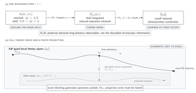
A Wilsonian step first integrates the shell $k/b<|p|<k$ and then rescales the remaining modes. The full trajectory is schematic and not to scale; the dashed projection onto a finite ansatz omits generated operators, while a field redefinition moves along a redundant coordinate direction rather than removing physical modes.

Dimensionless mass and quartic flow

Define dimensionless coordinates at the moving cutoff,

$$r(\ell)\equiv\frac{m^2(k)}{k^2}, \qquad u(\ell)\equiv K_d\lambda(k)k^{d-4}, \qquad \ell\equiv\ln\frac{\Lambda_{\rm UV}}{k}.$$

Combining the shell shifts with $b=e^{\delta\ell}$ gives one explicit step:

$$\begin{aligned} r(\ell+\delta\ell) &= r(\ell) +\left[ 2r+\frac{u}{2(1+r)} \right]\delta\ell +O(u^2\delta\ell,\delta\ell^2),\\ u(\ell+\delta\ell) &= u(\ell) +\left[ (4-d)u-\frac{3u^2}{2(1+r)^2} \right]\delta\ell +O(u^3\delta\ell,\delta\ell^2). \end{aligned}$$

Taking $\delta\ell\to0$ produces the flow stated in the lead. The $2r$ and $(4-d)u$ terms come only from rescaling; the rational terms come only from the shell integral. Keeping those sources separate prevents a dimensionful shell shift from being mistaken for a beta function.

At $d=4$ and $r=0$, $K_4=1/(8\pi^2)$. Since $d/d\ell=-d/d\ln k$, the quartic equation becomes

$$\frac{d\lambda}{d\ln k} = \frac{3\lambda^2}{16\pi^2}+O(\lambda^3),$$

which checks both the combinatorial factor and the RG-direction sign against the standard one-loop coefficient. For $d=4-\epsilon$, the projected non-Gaussian stationary point begins at

$$u_*=\frac{2\epsilon}{3}+O(\epsilon^2), \qquad r_*=-\frac{\epsilon}{6}+O(\epsilon^2).$$

The coordinates themselves depend on the cutoff and projection. The next chapter develops the invariant content extracted from linearized scaling exponents rather than from the numerical location of this point.

Composition and the semigroup check

Nested exact shell integrations compose. Eliminating $k/b_1<|p|<k$ and then $k/(b_1b_2)<|p|<k/b_1$ integrates the same variables as one step with $b=b_1b_2$. Including the matching rescalings gives

$$\mathcal T_{b_2}\circ\mathcal T_{b_1} = \mathcal T_{b_1b_2}.$$

For the autonomous projected flow $z=(r,u)$ and $dz/d\ell=\beta(z)$, an infinitesimal update is

$$\Phi_{\delta\ell}(z) = z+\delta\ell\,\beta(z)+O(\delta\ell^2).$$

Two updates therefore give

$$\Phi_{\delta\ell_2} \!\left(\Phi_{\delta\ell_1}(z)\right) = z+(\delta\ell_1+\delta\ell_2)\beta(z) +O(\delta\ell_1^2,\delta\ell_1\delta\ell_2,\delta\ell_2^2),$$

which agrees with one combined first-order step to the accuracy claimed. The $O(\delta\ell_1\delta\ell_2)$ term is not a failure of coarse graining; it is outside a first-order Euler update.

There is a separate projection issue. If $P$ retains only $r$ and $u$, then generally

$$P\mathcal T_{b_2}P\mathcal T_{b_1}P \ne P\mathcal T_{b_1b_2}P,$$

because operators discarded after the first step can feed back during the second. Exact shell maps form a semigroup; a repeatedly projected finite ansatz need not. This is why enlarging and testing a truncation is part of the result rather than optional numerical housekeeping.

Checks and limitations

• Gaussian limit. Setting $u=0$ leaves $dr/d\ell=2r$, the canonical mass scaling, while the field normalization remains fixed at this order.
• Dimensional check. $I_1$ has dimension $d-2$ and $I_2$ has dimension $d-4$, so $\lambda I_1$ has mass dimension two and $\lambda^2I_2$ has dimension $4-d$, matching $m^2$ and $\lambda$.
• Perturbative ceiling. The displayed mass flow omits $O(u^2)$ terms and the quartic flow omits $O(u^3)$ terms. It also sets the anomalous field rescaling to zero at the retained order.
• Sharp-cutoff ceiling. The local expansion is intended for external momenta below the shell. Momentum dependence near a sharp boundary requires more care; a smooth covariance leads to the functional flow on the next page.
• Projection ceiling. The two beta functions do not prove that the two-operator surface is invariant. Higher-field and derivative operators are generated even when they are canonically suppressed near four dimensions.

Common pitfalls

Reporting the shell shift as the full flow. The signs and powers in $\delta m^2$ and $\delta\lambda$ describe integration at fixed coordinates. A beta function for $r$ or $u$ also contains the canonical rescaling terms.

Changing the direction variable silently. Increasing $\ell$ lowers $k$. A beta function written with $\ln k$ has the opposite sign, so fixed-point stability labels cannot be transferred without declaring the direction.

Calling a projected recursion exact. The functional integration can be exact while the local expansion, perturbative cumulants, and $(r,u)$ projection are approximate. Generated operators must be retained or bounded before closure is claimed.

Exercises

For $m^2/k^2=r$, derive the thin-shell formula for $I_n$ directly from radial coordinates.

Solution

Using $d^dq=S_{d-1}q^{d-1}dq$,

$$I_n = K_d\int_{ke^{-\delta\ell}}^k \frac{q^{d-1}\,dq}{(q^2+m^2)^n}.$$

The interval has width $k\delta\ell+O(\delta\ell^2)$. Evaluating the smooth radial integrand at $q=k$ gives

$$I_n = K_d\frac{k^d}{(k^2+m^2)^n}\delta\ell +O(\delta\ell^2) = K_d\frac{k^{d-2n}}{(1+r)^n}\delta\ell +O(\delta\ell^2).$$

Translate the $d=4$, $r=0$ quartic flow from $u$ and $\ell$ to $\lambda$ and $\ln k$.

Solution

At $d=4$, $u=K_4\lambda=\lambda/(8\pi^2)$ and $du/d\ell=-3u^2/2$. Because $\ell=\ln(\Lambda_{\rm UV}/k)$,

$$\frac{d\lambda}{d\ln k} = -\frac{1}{K_4}\frac{du}{d\ell} = \frac32K_4\lambda^2 = \frac{3\lambda^2}{16\pi^2}.$$

Find the nonzero stationary point through first order in $\epsilon$.

Solution

Since $r_*=O(\epsilon)$, the quartic equation gives

$$0=\epsilon u_* -\frac32u_*^2+O(\epsilon^3),$$

so $u_*=2\epsilon/3+O(\epsilon^2)$. The mass equation then gives $0=2r_*+u_*/2+O(\epsilon^2)$ and hence $r_*=-\epsilon/6+O(\epsilon^2)$. Terms beyond these orders would not be controlled by the displayed truncation.

Explain why inserting a projection after each of two exact shell steps can spoil their composition law.

Solution

After the first exact step, write the action as retained coordinates plus an omitted component, $\mathcal T_{b_1}S=S_{r,u}+S_\perp$. The second exact step can mix $S_\perp$ back into the mass and quartic terms. Projecting immediately sets $S_\perp$ to zero, so the second step starts from different data. Thus $P\mathcal T_{b_2}P\mathcal T_{b_1}P$ need not equal $P\mathcal T_{b_1b_2}P$, even though the unprojected maps compose.

Continuations

• The Polchinski Exact RG Equation replaces the sharp infinitesimal shell by a smooth covariance and derives a functional flow without assuming two-coupling closure.
• Functional-RG Truncations and Projection Methods develops systematic ways to extract and test finite systems from a functional equation.
• Fixed Points, Universality, and Continuum Limits analyzes stationary trajectories, scaling fields, and universal exponents with the flow direction declared.

References

• Wilson, Kenneth G., and John Kogut. “The Renormalization Group and the $\epsilon$ Expansion.” Physics Reports 12 (1974): 75–199. DOI. Open PDF.