The Polchinski Exact RG Equation

Polchinski’s equation replaces a sequence of momentum shells by a smooth differential identity for a Wilsonian interaction functional. With the fixed field coordinate and covariance convention defined below, the equation is

$$\partial_t S_k^{\rm I} = \frac12 S_k^{{\rm I}(1)}\!\cdot D_k\cdot S_k^{{\rm I}(1)} -\frac12\operatorname{Tr}\!\left(D_kS_k^{{\rm I}(2)}\right), \qquad D_k\equiv\partial_tC_k,$$

where $t=\ln(k/\Lambda_{\rm UV})$. The product term joins two Wilson vertices, and the trace term contracts two legs of one vertex. Their balance makes the regulated low-momentum generating functional independent of $k$. The identity is exact for the declared regulator and boundary data; a finite vertex or derivative solution is not.

Required background. Momentum-Shell Integration and Rescaling supplies mode elimination, infrared and ultraviolet scale directions, induced operators, and the distinction between an exact shell map and a projected coupling flow.

A smooth covariance and a Wilson interaction

Use the momentum shorthand

$$\int_p \equiv \int\frac{d^dp}{(2\pi)^d}, \qquad f\cdot A\cdot g \equiv \int_p f(p)A(p)g(-p).$$

Choose a smooth cutoff profile $K(x)$ with $K(0)=1$, a low-momentum plateau, and rapid decay as $x\to\infty$. In this page,

$$C_k(p) = \frac{K(p^2/k^2)}{p^2+m^2}, \qquad t\equiv\ln\frac{k}{\Lambda_{\rm UV}}, \qquad D_k(p)\equiv\partial_tC_k(p).$$

Lowering $k$ moves toward the infrared and decreases $t$. For a monotone profile, $D_k$ is concentrated around $p^2\sim k^2$ and is nonnegative there. The mass and fixed kinetic normalization have been placed in $C_k$; all remaining interactions, including any additional quadratic vertex, belong to $S_k^{\rm I}[\phi]$.

The regulated functional is

$$Z_k[J] = \mathcal N_k \int\mathcal D\phi\, \exp\!\left[ -\frac12\phi\cdot C_k^{-1}\cdot\phi -S_k^{\rm I}[\phi] +J\cdot\phi \right].$$

The Gaussian normalization obeys

$$\partial_t\ln\mathcal N_k = -\frac12\operatorname{Tr}(C_k^{-1}D_k).$$

For the simplest source argument, take $J(p)$ to have support inside the plateau where $D_k(p)=0$. Then varying $k$ changes only the propagating modes above the external momentum range. A cutoff without an exact plateau requires the equivalent $k$-dependent source factors rather than silently treating $J$ as inert.

Polchinski uses a propagator multiplied by a smooth momentum profile, lowers its cutoff while changing the interaction Lagrangian, and proves that low-momentum functions remain fixed in Polchinski 1984, § 3, pp. 275–278.

Cutoff independence as a total derivative

Set

$$\mathcal A_k[\phi] = \frac12\phi\cdot C_k^{-1}\cdot\phi +S_k^{\rm I}[\phi].$$

At $J=0$, differentiation gives

$$\partial_t\mathcal A_k = -\frac12 \phi\cdot C_k^{-1}D_kC_k^{-1}\cdot\phi +\partial_tS_k^{\rm I}.$$

Now impose

$$\boxed{ \partial_t S_k^{\rm I} = \frac12 S_k^{{\rm I}(1)}\cdot D_k\cdot S_k^{{\rm I}(1)} -\frac12 \operatorname{Tr}\!\left(D_kS_k^{{\rm I}(2)}\right) }.$$

Here $S^{{\rm I}(1)}=\delta S^{\rm I}/\delta\phi$ and $S^{{\rm I}(2)}=\delta^2S^{\rm I}/\delta\phi\,\delta\phi$. Direct substitution reorganizes the integrand derivative as

$$\begin{aligned} \partial_t\!\left( \mathcal N_ke^{-\mathcal A_k} \right) = -\frac12\frac{\delta}{\delta\phi}\cdot \Bigl\{ D_k\cdot \bigl(C_k^{-1}\phi-S_k^{{\rm I}(1)}\bigr) \mathcal N_ke^{-\mathcal A_k} \Bigr\}. \end{aligned}$$

The regulated functional integral of this total derivative vanishes under the stated boundary assumptions. The same argument holds with the low-momentum source because $D_k\cdot J=0$. Thus $\partial_tZ_k[J]=0$ and the corresponding low-momentum functional derivatives are cutoff independent.

An equivalent compact form is

$$\partial_t e^{-S_k^{\rm I}} = -\frac12 \frac{\delta}{\delta\phi}\cdot D_k\cdot \frac{\delta}{\delta\phi} e^{-S_k^{\rm I}}.$$

If one instead defines $\dot C_k\equiv-\partial_tC_k$, the same convention reads $-\partial_tS_k^{\rm I}=S_k^{{\rm I}(1)}\cdot\dot C_k\cdot S_k^{{\rm I}(1)}/2-\operatorname{Tr}(\dot C_kS_k^{{\rm I}(2)})/2$. Writing the definition beside the dot is essential: changing only the symbol changes the apparent signs.

What the two terms do

The product term takes one functional derivative of each of two interaction vertices and joins the exposed legs with the differentiated covariance $D_k$. The trace term takes two derivatives of one vertex and contracts those legs. They are often called the classical or tree term and the quantum or loop term, respectively, but that vocabulary does not make the first term dispensable or the second perturbative. Both occur in the exact functional identity.

The figure places this Wilson-action flow beside the effective-average-action flow developed on the next page. Inspect the functional name, kernel, and $k\to0$ box in each column; only the right branch ends at the ordinary 1PI effective action. The dashed band is deliberately separate from both exact identities.

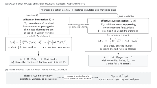
The solid branches are schematic exact identities for a regulated bosonic theory with $t=\ln(k/\Lambda_{\rm UV})$. Polchinski evolves the Wilsonian interaction $S_k^{\rm I}$ with covariance $C_k$; Wetterich evolves the modified Legendre functional $\Gamma_k$ with infrared kernel $R_k$. A compatible modified Legendre map can relate the descriptions, but the functionals and endpoints are not identical. The dashed $P_N$ layer is an additional truncation, so its finite trajectory is approximate.

The same relationships have the following text equivalent:

Question	Polchinski branch	Effective-average-action branch
Flowing object	Wilson interaction $S_k^{\rm I}[\phi]$ for fields still represented by $C_k$	Modified Legendre functional $\Gamma_k[\varphi]$ of the average field
Kernel	Multiplicative low-mode covariance $C_k$; its derivative transfers fluctuations into Wilson vertices	Additive infrared suppression $R_k$; its derivative releases fluctuations into $\Gamma_k$
Exact structure	Product of first derivatives minus a trace of the second derivative	One trace of the full inverse Hessian $(\Gamma_k^{(2)}+R_k)^{-1}$
Qualified infrared endpoint	$C_k(p)\to0$ at fixed nonzero $p$; $S_k^{\rm I}$ is not thereby the ordinary 1PI action	If $R_k\to0$ and the limit is controlled, $\Gamma_k\to\Gamma$
Where approximation enters	Vertex, momentum, or derivative projection of $S_k^{\rm I}$	Vertex, field, derivative, or polynomial projection of $\Gamma_k$

Wetterich derives the inverse-Hessian equation and its effective-action endpoint in Wetterich 1993, pp. 90–94. A modified Legendre relation requires compatible complementary kernels; the visual double arrow is not an equality of the two functionals at fixed arguments.

The exact vertex hierarchy

For a translation-invariant $\mathbb Z_2$ theory, expand

$$\begin{aligned} S_k^{\rm I}[\phi] = \sum_{\substack{n\ge0\\ n\ \text{even}}} \frac{1}{n!} \int_{p_1}\!\cdots\!\int_{p_n} &(2\pi)^d\delta^{(d)}\!\left(\sum_{i=1}^np_i\right)\\ &\times V_{n,k}(p_1,\ldots,p_n) \prod_{i=1}^n\phi(p_i). \end{aligned}$$

Let $A$ be a subset of the external labels, $B=A^c$, and $P_A=\sum_{i\in A}p_i$. Functional differentiation gives

$$\begin{aligned} \partial_tV_{n,k}(p_1,\ldots,p_n) =\;& \frac12 \sum_{\substack{A\subset\{1,\ldots,n\}\\ |A|,|B|\ \text{odd}}} V_{|A|+1,k}(p_A,-P_A) D_k(P_A)\\ &\qquad\times V_{|B|+1,k}(P_A,p_B)\\ &- \frac12\int_qD_k(q) V_{n+2,k}(q,-q,p_1,\ldots,p_n). \end{aligned}$$

The subset and its complement both occur in the sum, so the prefactor $1/2$ removes their double counting. This formula displays the infinite coupling explicitly: the product term partitions the external legs between two vertices, while the trace term makes $V_n$ depend on $V_{n+2}$.

Write $V_{2,k}(p,-p)=V_{2,k}(p)$. The first two equations are

$$\partial_tV_{2,k}(p) = D_k(p)V_{2,k}(p)^2 -\frac12\int_qD_k(q) V_{4,k}(p,-p,q,-q),$$

and

$$\begin{aligned} \partial_tV_{4,k}(p_1,p_2,p_3,p_4) =\;& \sum_{i=1}^4 D_k(p_i)V_{2,k}(p_i) V_{4,k}(p_1,p_2,p_3,p_4)\\ &- \frac12\int_qD_k(q) V_{6,k}(q,-q,p_1,p_2,p_3,p_4). \end{aligned}$$

At external momenta in the cutoff plateau, $D_k(p_i)=0$. The four-point flow is then controlled by the momentum-dependent six-point vertex. Setting $V_6=0$ merely because the microscopic action has no $\phi^6$ term erases the leading quartic loop flow.

Recovering the one-loop quartic coefficient

Take a massless four-dimensional theory in the scaling window $k\ll\Lambda_{\rm UV}$, with boundary data

$$V_{4,\Lambda}=\lambda, \qquad V_{n\ge6,\Lambda}=0.$$

To order $\lambda^2$, the $V_4V_4$ product in the six-point equation gives

$$\left.\partial_tV_{6,k}\right|_{\lambda^2} = \lambda^2 \sum_{\text{ten }3|3\text{ partitions}} D_k(P_A).$$

For arguments $(0,0,0,0,q,-q)$, six partitions carry momentum $q$ or $-q$ and four carry zero. Because $D_k(0)=0$ on the plateau, integration from the ultraviolet boundary gives

$$V_{6,k}(0,0,0,0,q,-q) = 6\lambda^2 \bigl[C_k(q)-C_{\Lambda}(q)\bigr] +O(\lambda^3).$$

Feeding this generated vertex into the four-point trace yields

$$\partial_t\lambda_k = 3\lambda_k^2 \int_qD_k(q) \bigl[C_{\Lambda}(q)-C_k(q)\bigr] +O(\lambda_k^3).$$

For the momenta selected by $D_k$, use $C_{\Lambda}(q)\simeq1/q^2$, $C_k(q)=K(x)/q^2$, and $x=q^2/k^2$. Since $D_k(q)=-2xK'(x)/q^2$,

$$\begin{aligned} \int_qD_k(q)\bigl[C_{\Lambda}(q)-C_k(q)\bigr] &= \frac{1}{8\pi^2} \int_0^\infty\frac{dq}{q} \bigl[-2xK'(x)\bigr]\bigl[1-K(x)\bigr]\\ &= \frac{1}{8\pi^2} \int_0^\infty dx\, \bigl[-K'(x)\bigr]\bigl[1-K(x)\bigr]\\ &= \frac{1}{16\pi^2}. \end{aligned}$$

Only $K(0)=1$ and $K(\infty)=0$ enter the last equality. Therefore

$$\boxed{ \frac{d\lambda_k}{d\ln k} = \frac{3\lambda_k^2}{16\pi^2} +O(\lambda_k^3) },$$

the same one-loop coefficient found by the thin-shell calculation. The functional hierarchy has reorganized the same three $s$, $t$, and $u$ bubble channels: it has not removed their intermediate momentum dependence.

Quasi-locality and field normalization

When $D_k(q)$ is smooth and concentrated at $q^2\sim k^2$, vertices evaluated at external momenta $|p_i|\ll k$ can be expanded in powers of $p_i/k$. That derivative expansion is the quasi-local representation of the Wilson action. It can fail near a non-smooth cutoff boundary, at singular field configurations, or when massless thresholds invalidate the expansion. The exact equation itself does not guarantee convergence of that representation.

The displayed flow uses a fixed field coordinate. If instead

$$C_k(p) = \frac{K(p^2/k^2)}{Z_k(p^2+m^2)},$$

then $D_k=\partial_tC_k$ must include $\partial_tZ_k$. Equivalently, define $\phi_R=Z_k^{1/2}\phi$, $\eta_k=-\partial_t\ln Z_k$, and $S_{R,k}[\phi_R]=S_k[Z_k^{-1/2}\phi_R]$. At fixed $\phi_R$, the chain rule adds

$$\left.\partial_tS_{R,k}\right|_{\phi_R} = \left.\partial_tS_k\right|_{\phi} +\frac{\eta_k}{2} \phi\cdot\frac{\delta S_k}{\delta\phi}.$$

Including $Z_k$ in the kernel and adding an independent field-rescaling term without a coordinate derivation would double count. Canonical momentum and field rescaling, needed for autonomous dimensionless fixed-point equations, is likewise an additional change of variables after the cutoff-compensation identity.

Checks and limitations

• Free theory. If $S_k^{\rm I}=0$, both terms vanish and the normalized Gaussian functional is $k$ independent for sources in the plateau.
• Symmetry. If the boundary functional is even in $\phi$ and $C_k$ is field independent, every term in the hierarchy preserves $\mathbb Z_2$.
• Vacuum terms. The hierarchy includes the field-independent vertex $V_{0,k}$. It may instead be absorbed into an additional $k$-dependent normalization, but it must be retained when a free energy or absolute normalization is the observable.
• Exactness ceiling. The derivation is a regulated functional-integration identity. It is not a proof that an infinite-dimensional trajectory exists globally or that a proposed continuum limit is constructive.
• Projection ceiling. Retaining $V_2$, $V_4$, and the full $O(\lambda^2)$ momentum dependence of $V_6$ is sufficient for the displayed one-loop check. Replacing those functions by finitely many numbers is a further approximation that needs its own error test.

Common pitfalls

Using $\dot C_k$ without defining it. Some authors set $\dot C_k=\partial_tC_k$ and others set $\dot C_k=-\partial_tC_k$. Derive the signs from $Z_k$ or state the definition next to the equation.

Truncating before the loop closes. A microscopic $V_6=0$ does not imply a flowing $V_6=0$. The $V_4V_4$ product generates it, and its trace supplies the one-loop $V_4$ flow.

Confusing a Wilson action with a 1PI action. $S_k^{\rm I}$ contains vertices for modes represented by $C_k$ and obeys a product-minus-trace equation. The ordinary effective action is the endpoint of the distinct modified Legendre construction on the next page.

Exercises

Verify the total-derivative identity at $J=0$, including the derivative of $\mathcal N_k$.

Solution

Let $a=C_k^{-1}\phi$ and $s=S_k^{{\rm I}(1)}$. Differentiating the normalized integrand and inserting the flow gives

$$\left[ -\frac12\operatorname{Tr}(C_k^{-1}D_k) +\frac12a\cdot D_k\cdot a -\frac12s\cdot D_k\cdot s +\frac12\operatorname{Tr}(D_kS_k^{{\rm I}(2)}) \right] \mathcal N_ke^{-\mathcal A_k}.$$

Expanding

$$-\frac12\frac{\delta}{\delta\phi}\cdot \left[D_k\cdot(a-s)\mathcal N_ke^{-\mathcal A_k}\right]$$

produces exactly the same four terms: the mixed $a\cdot D_k\cdot s$ terms cancel because $D_k$ is symmetric. Its regulated functional integral vanishes.

Derive the displayed two-point vertex equation from the general hierarchy.

Solution

For $n=2$, the only allowed subsets have one external label. The two complementary choices are equal and the prefactor $1/2$ leaves one product, $D_k(p)V_{2,k}(p)^2$. The trace term always appends $q,-q$ and therefore contains $V_{4,k}(p,-p,q,-q)$ with coefficient $-1/2$.

Evaluate the cutoff-profile integral in the one-loop check without choosing a particular $K(x)$.

Solution

Use $dq/q=dx/(2x)$. The radial integral becomes

$$\frac{1}{8\pi^2} \int_0^\infty dx\,[-K'(x)][1-K(x)] = \frac{1}{16\pi^2} \left[(1-K(x))^2\right]_{0}^{\infty}.$$

The boundary values $K(0)=1$ and $K(\infty)=0$ give $1/(16\pi^2)$. Smooth deformations of the profile do not change this one-loop coefficient under the stated assumptions.

Continuations

• Effective Average Actions and the Wetterich Equation derives the modified Legendre transform and the full inverse-Hessian trace shown in the right branch of the figure.
• Functional-RG Truncations and Projection Methods turns exact functional identities into finite systems with explicit closure and enlargement tests.
• Rigorous RG as a Dynamical System states theorem-level hypotheses for treating renormalization as an infinite-dimensional flow.

References

• Polchinski, Joseph. “Renormalization and Effective Lagrangians.” Nuclear Physics B 231 (1984): 269–295. DOI.
• Wetterich, Christof. “Exact Evolution Equation for the Effective Potential.” Physics Letters B 301 (1993): 90–94. DOI. Open PDF.