Local Field Redefinitions and the Equivalence Theorem

A field redefinition changes the coordinates used to describe a quantum field theory, not its physical scattering data—provided the map is local, perturbatively invertible, and implemented in the action, measure, sources, counterterms, and EFT truncation. The equivalence theorem is therefore a conditional statement about observables. It does not say that off-shell Green functions, Wilson coefficients, field residues, or boundary data remain numerically unchanged.

Required background. Integration by Parts and Equation-of-Motion Redundancy derives the order-by-order EOM reduction. LSZ Reduction: Poles, Residues, and Stable External States supplies the pole and amputation argument. Helpful background. Changes of Variables and Regulated Jacobians explains why the functional measure must be transformed with the fields.

The equivalence theorem

Let a regulated theory be described by fields $\Phi_i$ and action $S[\Phi]$. Consider

$$\Phi_i=F_i[\Phi'] =\Phi_i'+\epsilon G_i[\Phi'],$$

where $G_i$ is local and contains finitely many derivatives at each retained order. Treat every term proportional to $\epsilon$ perturbatively. Then the inverse exists as a local formal series,

$$\Phi_i' =\Phi_i-\epsilon G_i[\Phi]+O(\epsilon^2).$$

Statement. Suppose the transformation and its perturbative inverse preserve the field domain and boundary conditions; the regulated Jacobian and counterterms are included; the transformed fields retain nonzero overlap with the same stable one-particle states; and the action is expanded consistently through the target order. Then the original and transformed descriptions give the same $S$-matrix elements and physical observables through that order after their parameters are related by the induced coefficient map.

This is the EFT form of the change-of-field theorem proved in Kamefuchi, O’Raifeartaigh, and Salam 1961, pp. 529–549. Derivative-dependent local transformations and their use in reduced effective Lagrangians are treated in Arzt 1995, § 2, preprint pp. 4–7, Open PDF.

The assumptions can be checked individually:

Hypothesis	What it excludes	Required response if it fails
Locality order by order	Kernels with long-range support or inverse differential operators	Demonstrate observable equivalence by another argument; do not invoke the local theorem
Perturbative invertibility	Singular maps, projections, or changes in the number of field configurations	Treat the map as a different theory or coordinate patch
Same asymptotic poles	Loss of overlap with a stable external state or a resummed spurious pole	Choose valid interpolating fields and compare the physical pole spectrum
Complete transformed measure	A discarded nontrivial Jacobian or anomaly contribution	Retain the regulated Jacobian and its local terms
Consistent truncation	Missing interactions generated at the next retained power	Expand the map and action to the requested EFT order
Compatible boundary data	A surface term or transformed boundary condition that carries physics	Transform the boundary action and admissible data explicitly

The theorem applies cleanly to stable asymptotic particles. An unstable resonance is not an external LSZ state; compare amplitudes for its stable production and decay products, or compare a properly defined pole observable instead.

Why the path integral and LSZ agree

With a source $J_i$ coupled to the original field,

$$Z[J] =\int\mathcal D\Phi\, e^{iS[\Phi]+iJ_i\Phi_i}.$$

Changing variables gives the exact regulated identity

$$Z[J] =\int\mathcal D\Phi'\, \det\!\left(\frac{\delta F}{\delta\Phi'}\right) e^{iS[F(\Phi')]+iJ_iF_i(\Phi')}.$$

Thus the complete generating functional is unchanged when the action, determinant, and source composite $F_i(\Phi')$ are transformed together. If one instead couples $J_i$ directly to $\Phi_i'$, one generates different off-shell Green functions. That difference is expected: $\Phi$ and $\Phi'$ are different interpolating operators.

For a stable particle $a$, suppose

$$\langle0|\Phi_i(0)|a,p\rangle=Z_{ia}^{1/2}\ne0.$$

A perturbative transformation changes the residue continuously,

$$\langle0|F_i(\Phi')(0)|a,p\rangle =Z_{ia}^{1/2}+O(\epsilon),$$

but cannot move the physical pole or remove the overlap at sufficiently small $\epsilon$. LSZ divides by the appropriate residues and amputates the external poles. Local source differences and EOM insertions have fewer than the full set of one-particle poles, so they vanish after all external legs are reduced. Criado and Pérez-Victoria give this path-integral and pole-residue argument in Criado and Pérez-Victoria 2019, § 2, pp. 5–9, Open PDF.

There are two important qualifications. First, for

$$F(\Phi')=\Phi'+\epsilon G(\Phi'),$$

the determinant may be represented by local ghost fields. In dimensional regularization, closed ghost loops from a local perturbative map are polynomial momentum integrals and vanish under the usual assumptions. Other regulators can leave local Jacobian terms, and anomaly-producing transformations require their own regulated analysis.

Second, higher-derivative quadratic terms created by the map remain perturbative interactions. Resumming them into a propagator can manufacture extra poles that were absent order by order. The theorem relates the perturbative expansions, not an uncontrolled resummation of one representation.

Quotient classes and representative changes

A redundant EOM operator is tangent to a field-coordinate orbit at the working order. The quotient identifies that direction, while a field redefinition constructs an explicit path from one representative action to another.

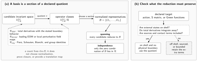
An operator basis is a normalized section of a quotient, not the unreduced candidate list or its count. Panel (a) forms classes in $\mathcal V_{d,\mathbf q}^{\mathrm{inv}}/\mathcal R$, chooses representatives, and tests spanning and independence separately. Panel (b) limits the reduction: on-shell observables with boundary conditions that remove total derivatives use the quotient, whereas off-shell Green functions, explicit sources and contact terms, or physical boundaries can require the extra operators. The diagram is schematic and not to scale.

If $S=S_0+\epsilon S_1+\epsilon^2S_2+\cdots$, the first-order map changes

$$S_1\longmapsto S_1+G_i\frac{\delta S_0}{\delta\Phi_i}.$$

At second order it also generates

$$G_i\frac{\delta S_1}{\delta\Phi_i} +\frac12G_iG_j \frac{\delta^2S_0}{\delta\Phi_i\delta\Phi_j},$$

plus the contribution of any explicit second-order field map. Therefore the leading EOM is sufficient to remove a first-order operator, but it is not sufficient to reconstruct the transformed action two orders later. A precise order-by-order workflow and examples of the missed terms appear in Criado and Pérez-Victoria 2019, §§ 3 and 5.1, pp. 9–12 and 16–18, Open PDF.

First application: a derivative scalar interaction

Take a real scalar with

$$\mathcal L =\frac12(\partial\phi)^2 -\frac12m^2\phi^2 -\frac{g}{4!}\phi^4 +\frac{c}{\Lambda^2}\phi^2(\partial\phi)^2 +O(\Lambda^{-4}).$$

Use the local map

$$\phi =\chi-\frac{c}{3\Lambda^2}\chi^3.$$

Direct expansion of the lower-order Lagrangian gives

$$\begin{aligned} \delta\mathcal L_0 ={}&-\frac{c}{\Lambda^2} \chi^2(\partial\chi)^2 +\frac{cm^2}{3\Lambda^2}\chi^4\\ &+\frac{cg}{18\Lambda^2}\chi^6 +O(\Lambda^{-4}). \end{aligned}$$

The derivative interaction cancels, leaving

$$\mathcal L' =\frac12(\partial\chi)^2 -\frac12m^2\chi^2 -\frac{g}{4!}\chi^4 +\frac{cm^2}{3\Lambda^2}\chi^4 +\frac{cg}{18\Lambda^2}\chi^6 +O(\Lambda^{-4}).$$

The two Lagrangians look different, and individual Wilson coefficients have changed. Their on-shell four-point amplitudes nevertheless agree. With all momenta incoming, the derivative vertex polynomial, after symmetrizing the two differentiated fields, is

$$V_{\partial} =-4c\sum_{i<j}p_i\cdot p_j.$$

Momentum conservation and $p_i^2=m^2$ imply

$$\sum_{i<j}p_i\cdot p_j =\frac12\left[ \left(\sum_i p_i\right)^2-\sum_i p_i^2 \right] =-2m^2,$$

so $V_{\partial}=8cm^2$. In the transformed theory, the induced contact $(cm^2/3)\chi^4$ gives

$$V_{\mathrm{red}} =4!\frac{cm^2}{3} =8cm^2.$$

The common factor $i/\Lambda^2$ and the unchanged leading amplitude have been suppressed. This is a nontrivial equality: in the massless limit both corrections vanish, while for $m\ne0$ the field redefinition trades momentum dependence for a local potential term.

At six points, the induced $cg\chi^6/18$ vertex is essential. It combines with diagrams containing the shifted four-field interaction to reproduce diagrams containing the original derivative vertex and one ordinary $g\phi^4$ interaction. Comparing only the six-point contact terms would not test the theorem.

Where the theorem does not apply directly

Nonlocal transformations. A map such as $\Phi'=(\Box+m^2)^{-1}\Phi$ changes pole structure and long-distance support. Local-EFT equivalence does not follow.

Noninvertible maps. The map $\Phi=(\Phi')^2$ is singular at the origin and is not one-to-one. It changes the integration domain and cannot be treated as a harmless coordinate change.

Changed boundaries. A derivative transformation can alter both boundary values and normal derivatives. The transformed boundary action and admissible data must be supplied before observables can be compared.

Anomalous measure transformations. A classical symmetry transformation with a nontrivial regulated Jacobian generates a physical local term. Including that term preserves the change-of-variables identity; discarding it gives the wrong theory.

Unstable external particles. LSZ assumes stable one-particle poles. For a resonance, formulate the observable with stable asymptotic states rather than declaring an external unstable-particle amplitude invariant.

Common pitfalls

Transforming only the displayed operator. The lower-order action, higher-order terms, sources, counterterms, gauge-fixing sector, and measure all respond to the map. Retain every response that enters the target accuracy.

Comparing Wilson coefficients as observables. A coefficient is a coordinate dual to a chosen operator representative. Compare matched amplitudes, pole quantities, or other physical observables after applying the full coefficient map.

Resumming a perturbative derivative map. An exact-looking modified propagator can add spurious degrees of freedom. Expand consistently in $1/\Lambda$.

Claiming off-shell invariance. The exact generating functional is invariant only when its composite source coupling is transformed. Green functions of the new elementary coordinate are generally different.

Exercises

Verify the factor $-4$ in the scalar derivative vertex.

Solution

Choose which two of the four external legs occupy the differentiated factors. For each unordered pair, the two differentiated slots and the two undifferentiated slots each contribute a factor $2!$, while the derivatives contribute $(-i)^2p_i\cdot p_j=-p_i\cdot p_j$. Thus the fourfold multiplicity gives $-4\sum_{i<j}p_i\cdot p_j$.

Consider $\phi=\chi+\epsilon\Box\chi$. Why is its inverse local only perturbatively?

Solution

Order by order,

$$\chi =\phi-\epsilon\Box\phi +\epsilon^2\Box^2\phi-\cdots,$$

and every retained term contains finitely many derivatives at one point. The formally resummed inverse $(1+\epsilon\Box)^{-1}$ is a Green-function kernel with nonlocal support and additional pole structure. The local equivalence theorem applies to the truncated series, not automatically to that resummation.

References

• Arzt, Christopher. “Reduced Effective Lagrangians.” Physics Letters B 342, no. 1–4 (1995): 189–195. DOI; Open PDF
• Criado, Juan Carlos, and Manuel Pérez-Victoria. “Field Redefinitions in Effective Theories at Higher Orders.” Journal of High Energy Physics 2019, no. 3 (2019): 038. DOI; Open PDF
• Kamefuchi, S., L. O’Raifeartaigh, and A. Salam. “Change of Variables and Equivalence Theorems in Quantum Field Theories.” Nuclear Physics 28 (1961): 529–549. DOI