Evolution Kernels, Consistency Relations, and Resummation Architecture

Factorization replaces one badly behaved fixed-order expression by several functions, each with its own natural scale. Renormalization-group evolution transports those boundary functions to a common scale. The transport resums logarithms only if the anomalous dimensions satisfy the same consistency relations as the factorization formula, and only if fixed-order boundary terms are not counted again in the evolved result.

This page builds that architecture for the off-shell Sudakov product. Its four cusp kernels reproduce the leading double logarithm and provide an exact common-scale cancellation test. Matrix evolution, logarithmic accuracy, profile scales, and fixed-order matching then extend the construction beyond this scalar kernel example.

Required background. Matching onto Factorized Operator Structures supplies the hard, collinear, and soft factors. Dual Evolution of Operators and Wilson Coefficients supplies coefficient–operator sign and transpose conventions. Large Logarithms and RG Improvement supplies the single-scale evolution logic.

Helpful background. Sudakov Logarithms and Resummation develops observable-level applications.

Consistent kernels for the Sudakov product

Consider an amplitude-level factorization with two off-shell collinear legs,

$$F(Q^2,L^2,P^2) =C(Q^2,\mu) J_L(L^2,\mu) J_P(P^2,\mu) S(\Lambda_s^2,\mu), \qquad \Lambda_s^2=\frac{L^2P^2}{Q^2}.$$

Write $\Gamma(\alpha_s)=C_F\gamma_{\mathrm{cusp}}(\alpha_s)$. The multiplicative RG equations have the form

$$\begin{aligned} \frac{d\ln C}{d\ln\mu} &=\Gamma\ln\frac{Q^2}{\mu^2}+\gamma_C, \\ \frac{d\ln J_L}{d\ln\mu} &=-\Gamma\ln\frac{L^2}{\mu^2}+\gamma_{J_L}, \\ \frac{d\ln J_P}{d\ln\mu} &=-\Gamma\ln\frac{P^2}{\mu^2}+\gamma_{J_P}, \\ \frac{d\ln S}{d\ln\mu} &=\Gamma\ln\frac{\Lambda_s^2}{\mu^2}+\gamma_S. \end{aligned}$$

The cusp logarithms sum to zero because

$$\ln\frac{Q^2}{\mu^2} -\ln\frac{L^2}{\mu^2} -\ln\frac{P^2}{\mu^2} +\ln\frac{\Lambda_s^2}{\mu^2}=0.$$

The noncusp terms must independently satisfy

$$\gamma_C+\gamma_{J_L}+\gamma_{J_P}+\gamma_S=0.$$

These are not optional simplifications. They express $dF/d\ln\mu=0$ and test the scale relation, operator renormalization, zero-bin assignments, and sign conventions simultaneously.

Factor	Natural virtuality scale	Cusp sign	Boundary calculation
$C(Q^2)$	$\mu_h=Q$	$+$	Hard matching with no large $\ln(Q^2/\mu_h^2)$
$J_L(L^2)$	$\mu_L=\sqrt{L^2}$	$-$	First collinear sector
$J_P(P^2)$	$\mu_P=\sqrt{P^2}$	$-$	Second collinear sector
$S(\Lambda_s^2)$	$\mu_s=\sqrt{\Lambda_s^2}=\sqrt{L^2P^2}/Q$	$+$	Ultrasoft Wilson-line matrix element

Becher, Broggio, and Ferroglia derive these equations and their consistency sum in Becher, Broggio, and Ferroglia 2015, §§ 5.1–5.2, preprint pp. 48–53, Open PDF.

In an early SCET endpoint calculation, the soft and collinear contributions are both needed to reproduce the full theory’s infrared behavior; matching is free of the large logarithm at its natural scale, and coefficient evolution then sums the Sudakov series. See Bauer, Fleming, and Luke 2000, §§ III.B–III.C, preprint pp. 11–13, Open PDF.

Evolution operators and path ordering

For a column vector of renormalized functions obeying

$$\frac{d}{d\ln\mu}\mathbf F(\mu) =\boldsymbol\gamma(\mu)\mathbf F(\mu),$$

the solution is

$$\mathbf F(\mu) =\mathbf U(\mu,\mu_0)\mathbf F(\mu_0), \qquad \mathbf U(\mu,\mu_0) =P\exp\!\left[ \int_{\mu_0}^{\mu}\frac{d\mu'}{\mu'} \boldsymbol\gamma(\mu') \right].$$

Path ordering is required when

$$[\boldsymbol\gamma(\mu_1),\boldsymbol\gamma(\mu_2)]\ne0.$$

Dropping $P$ is justified only after proving commutativity or diagonalizing in a scale-independent basis. A valid kernel also obeys

$$\mathbf U(\mu_2,\mu_1) \mathbf U(\mu_1,\mu_0) =\mathbf U(\mu_2,\mu_0), \qquad \mathbf U^{-1}(\mu,\mu_0)=\mathbf U(\mu_0,\mu).$$

These composition tests catch ordering and transpose errors that can remain invisible in a first-order expansion.

For a commuting cusp kernel, change variables from scale to coupling. Define

$$a_\gamma(\nu,\mu) =-\int_{\alpha_s(\nu)}^{\alpha_s(\mu)} d\alpha\,\frac{\gamma(\alpha)}{\beta(\alpha)},$$

and

$$S_\Gamma(\nu,\mu) =-\int_{\alpha_s(\nu)}^{\alpha_s(\mu)} d\alpha\,\frac{\Gamma(\alpha)}{\beta(\alpha)} \int_{\alpha_s(\nu)}^\alpha \frac{d\alpha'}{\beta(\alpha')}.$$

The hard-amplitude kernel can then be written

$$U_C(\mu,\mu_h) =\exp\!\left[ 2S_\Gamma(\mu_h,\mu) -a_{\gamma_C}(\mu_h,\mu) \right] \left(\frac{Q^2}{\mu_h^2}\right)^{-a_\Gamma(\mu_h,\mu)}.$$

Analogous kernels with their own cusp signs and physical arguments evolve the jets and soft function. Expanding a kernel to its input order must reproduce the original RGE and its boundary value $U_i(\mu_i,\mu_i)=1$.

First application: reproduce the leading Sudakov exponent

Freeze $\alpha_s$, keep only the one-loop cusp term, and set all noncusp anomalous dimensions to zero. Let

$$\Gamma=\Gamma_0\frac{\alpha_s}{4\pi}$$

be constant. Evolve each factor from its natural scale in the table to an arbitrary common $\mu$. Direct integration gives

$$\begin{aligned} \ln\frac{F_{\mathrm{LL}}}{F_{\mathrm{boundary}}} =-\Gamma\bigg[ &\ln^2\frac{Q}{\mu} -\ln^2\frac{\sqrt{L^2}}{\mu} -\ln^2\frac{\sqrt{P^2}}{\mu} \\ &+\ln^2\frac{\sqrt{L^2P^2}/Q}{\mu} \bigg]. \end{aligned}$$

Using $\sqrt{\Lambda_s^2}=\sqrt{L^2P^2}/Q$, every dependence on the arbitrary common scale cancels, leaving

$$\boxed{ F_{\mathrm{LL}} =F_{\mathrm{boundary}} \exp\!\left[ -\frac{\Gamma}{2} \ln\frac{Q^2}{L^2} \ln\frac{Q^2}{P^2} \right] }.$$

For a quark current, $\Gamma_0=4C_F$, so

$$F_{\mathrm{LL}} =F_{\mathrm{boundary}} \exp\!\left[ -\frac{C_F\alpha_s}{2\pi} \ln\frac{Q^2}{L^2} \ln\frac{Q^2}{P^2} \right].$$

This is the leading off-shell Sudakov suppression. The derivation uses all four factors: deleting the soft kernel or assigning it the jet sign leaves a spurious $\mu$ dependence and the wrong exponent. Running coupling promotes the simple squares to $S_\Gamma$ and $a_\Gamma$ integrals without changing the consistency test. For a cross section, the hard boundary is $H=|C|^2$ and the amplitude exponent is combined with the corresponding measured jet and soft functions.

Declaring logarithmic accuracy

An accuracy label is meaningful only with an ingredient convention. A common exponent-counting convention is:

Accuracy	Cusp anomalous dimension	Noncusp anomalous dimensions	$\beta$ function	Boundary matching
LL	1 loop	omitted	1 loop	tree
NLL	2 loops	1 loop	2 loops	tree
NLL$'$	2 loops	1 loop	2 loops	1 loop
NNLL	3 loops	2 loops	3 loops	1 loop

The prime adds one order of fixed boundary terms without increasing the evolution order. Other communities shift labels, so a result should list ingredients rather than rely on “NLL” alone. Matrix problems must additionally state the perturbative order and basis used for diagonalization or path ordering.

Boundary functions are evaluated at natural scales and then evolved; their fixed-order logarithms must not be added a second time. When a resummed prediction is combined with a full fixed-order result, additive matching through order $k$ is

$$\sigma_{\mathrm{match}} =\sigma_{\mathrm{res}} +\sigma_{\mathrm{FO}}^{(k)} -\left[\sigma_{\mathrm{res}}\right]_{\mathrm{expanded}}^{(k)}.$$

The subtraction must use the same conventions, inputs, phase space, and distributions as the fixed-order term. Its expansion is an essential reproduction test, not merely bookkeeping.

Canonical scales, profiles, and uncertainty

Canonical scales minimize logarithms in each boundary function. For a two-jet distribution with small event shape $\tau$, a typical hierarchy is

$$\mu_H\sim Q, \qquad \mu_J\sim Q\sqrt{\tau}, \qquad \mu_S\sim Q\tau.$$

A fixed canonical choice can enter the nonperturbative region as $\tau\to0$ and can continue resumming where the singular and nonsingular terms are comparable. Profile scales replace it with smooth functions of $\tau$ that:

• freeze the soft scale above a declared perturbative floor;
• follow canonical scaling in the resummation region;
• merge $\mu_J$ and $\mu_S$ into $\mu_H$ where fixed order should take over; and
• remain ordered and differentiable through the transition regions.

Uncertainty should retain its origin. Vary the hard, jet, and soft boundary scales around their canonical values subject to the hierarchy; vary profile transition points and curvature; vary the common evolution scale as a correlation check; and compare the matched expansion with the exact fixed-order result. The envelope is a truncation diagnostic, not a statistical confidence interval. A profile that crosses a Landau pole or creates a new large logarithm is inadmissible rather than an uncertainty variation.

The evolution stage in the construction map

The last numbered box in the right panel represents the kernel architecture developed here. Its separate $\mu$ and $\nu$ labels matter: this page evolves virtuality. The next page adds rapidity evolution when equal-virtuality modes cannot be separated by $\mu$ alone.

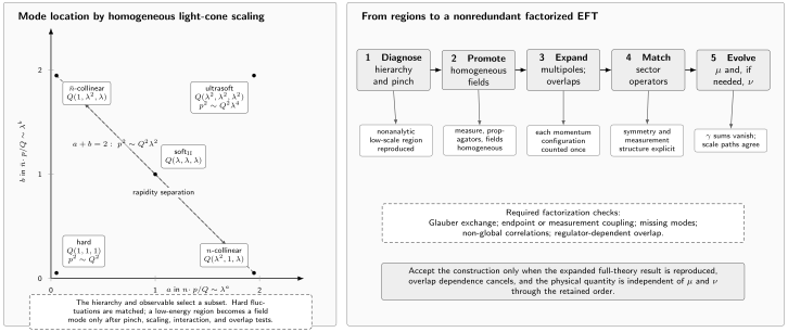
Mode locations are shown in the exponents $a$ and $b$ of $(n\!\cdot p/Q,\bar n\!\cdot p/Q)\sim(\lambda^a,\lambda^b)$, with the transverse exponent written in each label. The line $a+b=2$ contains $n$-collinear, $\bar n$-collinear, and soft-II scalings of virtuality $Q^2\lambda^2$; their separation along the line is a rapidity separation. Ultrasoft momentum has virtuality $Q^2\lambda^4$, while hard fluctuations are matched at $Q^2$. The points are alternatives selected by a hierarchy and observable, not a universal simultaneous field list. A consistent construction requires homogeneous fields, multipole and overlap expansion, sector matching, and $\mu$ and, when needed, $\nu$ evolution, with explicit factorization checks. The diagram is schematic and not to scale.

Common pitfalls

Evolving every factor from the hard scale. Jets and soft functions have lower natural scales. Starting all boundaries at $Q$ leaves the logarithms inside fixed-order matching instead of resumming them through controlled kernels.

Dropping path ordering by inspection. A matrix that is diagonal at one scale need not share eigenvectors at another. Check commutators or solve the ordered system directly.

Using scale variation to hide inconsistency. If the anomalous-dimension sum is nonzero, no scale choice repairs the factorization formula. Locate the missing mode, overlap, operator, or counterterm first.

Adding resummed and fixed-order results without subtraction. Their common expansion is then counted twice. Verify the matched result through the declared fixed order before using it outside the asymptotic region.

Exercises

1. Why does a cusp term in an anomalous dimension produce double logarithms?

   Solution

   The cusp term already contains a logarithm such as $\ln(Q/\mu)$. Integrating the RG equation over $\mathrm d\ln\mu$ therefore produces $\ln^2(Q/\mu)$; coupling running organizes the higher logarithmic towers.

2. What is the strongest fixed-order check of a resummed expression?

   Solution

   Expand the resummed result to the known order and compare every singular distribution, logarithm, and scale-dependent constant with the fixed-order calculation in identical conventions.

References

• Bauer, Christian W., Sean Fleming, and Michael Luke. 2000. “Summing Sudakov Logarithms in $B\to X_s\gamma$ in Effective Field Theory.” Physical Review D 63 (1): 014006. DOI. Open PDF.

• Becher, Thomas, Alessandro Broggio, and Andrea Ferroglia. 2015. Introduction to Soft-Collinear Effective Theory. Lecture Notes in Physics 896. Cham: Springer. DOI. Open PDF.