Matching Conditions Beyond Tree Level

Loop matching determines the short-distance part of a renormalized full-theory calculation that is not already generated by the EFT. The operative equation is therefore not “full loop equals Wilson coefficient,” but “full theory equals EFT” for the same matching object, external data, fields, scheme, scale, and infrared prescription. Expanding this equality order by order makes the common low-energy contribution cancel and leaves a local hard coefficient.

Required background. Tree-Level Matching and Classical Elimination fixes the lower-order coefficients inserted in EFT loops. Local Counterterms and Subdivergence Structure supplies the locality of renormalized short-distance subtractions. Observable, Off-Shell, Background-Field, and Functional Matching fixes what is being compared. Helpful background. Scheme Transformations and RG Invariants explains finite parameter and operator-coordinate changes.

The renormalized matching equation

Choose renormalized quantities $\mathcal F_a$—for example projected amplitudes or 1PI vertices—whose tree-level response to the target operators is the matrix $R_{ai}$. Write the Wilson coefficients as

$$C_i(\mu_m) = C_i^{(0)}(\mu_m) +\frac{1}{16\pi^2}C_i^{(1)}(\mu_m) +\cdots,$$

where $\mu_m$ is the matching scale. After the full-theory parameters and light fields have been expressed in the EFT convention, the one-loop expansions have the form

$$\begin{aligned} \mathcal F_{a,\mathrm{full}}^{\mathrm{ren}} &=\mathcal F_a^{(0)} +R_{ai}C_i^{(0)} +\frac{1}{16\pi^2} \left(H_a+S_a\right),\\ \mathcal F_{a,\mathrm{EFT}}^{\mathrm{ren}} &=\mathcal F_a^{(0)} +R_{ai}C_i^{(0)} +\frac{1}{16\pi^2} \left(R_{ai}C_i^{(1)}+S_a\right). \end{aligned}$$

$S_a$ denotes the light-momentum or infrared part common to both theories. In the EFT it is produced by loops containing the already matched $C_i^{(0)}$ and ordinary light interactions. $H_a$ is analytic in the retained external momenta and light masses around the matching point, so it can be represented by local operators. Equality of the two renormalized calculations gives

$$\boxed{R_{ai}C_i^{(1)}=H_a}$$

through the requested order. If $R$ is square and nonsingular, this equation can be inverted directly. More generally, the matching data must span the desired coefficient combinations; unused projections then become independent checks. The functional version equates the light-particle-irreducible effective actions and yields the same subtraction Henning, Lu, and Murayama 2016, §§ 1–2, pp. 2–17, PDF.

The figure’s second panel depicts this equation. The shared infrared term belongs to neither Wilson coefficient: it cancels only after the two calculations have been aligned.

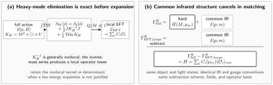
Heavy-field elimination and matching separate two steps. Panel (a) integrates a Gaussian heavy field with quadratic operator $K_H=M^2+\Box+U[\phi]$ and light source $J[\phi]$, producing an exact, generally nonlocal source term and a field-dependent determinant; only for $Q/M\ll1$ are these expanded into local operators. Panel (b) shows a renormalized loop matching condition: with the matching object, light states, infrared prescription, gauge, scheme, fields, and basis aligned, the common infrared term cancels and the remainder fixes the hard Wilson coefficients. The diagram is schematic and not to scale.

What must be included at one loop

The compact symbols $H_a$ and $S_a$ hide several terms that are easy to omit. A one-loop matching equation at fixed EFT order includes:

1. renormalized full-theory one-loop graphs, including pure-heavy and mixed heavy–light topologies;
2. full-theory counterterm insertions and the conversion of full parameters to the chosen renormalized inputs;
3. EFT one-loop graphs built from the leading light Lagrangian and every lower-order Wilson coefficient that can contribute;
4. EFT counterterm insertions, including operator mixing and evanescent sectors when present;
5. finite light-field, mass, coupling, tadpole, and external-residue maps required to put both sides in the same coordinates; and
6. the new local coefficient $C_i^{(1)}$ multiplying its tree matrix element.

Loop order and inverse-scale order are independent labels. A loop containing a dimension-six tree coefficient can contribute at the same requested accuracy as a one-loop dimension-six matching coefficient. Conversely, a pure-heavy loop may first generate an operator that was absent at tree level. The bookkeeping should therefore label every term by loop order, coupling order, and EFT order rather than by a single word such as “next-to-leading.”

A method-of-regions calculation makes the cancellation transparent. For a full integral depending on a heavy mass $M$ and light data $(Q,m)$,

$$I_{\mathrm{full}}(Q,m,M) = I_{\mathrm{hard}}(M;Q,m) +I_{\mathrm{soft}}(Q,m;M),$$

where each term is expanded homogeneously to the target order. The EFT graph obtained by expanding the heavy propagator before integration reproduces $I_{\mathrm{soft}}$. Thus

$$I_{\mathrm{full}}-I_{\mathrm{EFT}} = I_{\mathrm{hard}},$$

including the region counterterms and overlap prescription. The right side is a polynomial in the low-energy data at any fixed order. Beneke and Smirnov formulate region expansions as homogeneous Taylor expansions associated with graph substructures in Beneke and Smirnov 1998, pp. 321–344. Detailed ultraviolet-versus-infrared pole bookkeeping is deferred to Infrared Consistency in Matching.

A pure-heavy one-loop coefficient

Use the chapter’s real light scalar $\phi$ and heavy scalar $H$, now with the quadratic portal

$$\mathcal L \supset -\frac12M^2H^2 -\frac{\kappa}{4}H^2\phi^2.$$

Set the linear coupling $g$ of the tree-level example to zero for this benchmark, and take the light theory to be free apart from the operators being matched. The field-dependent heavy mass is

$$m_H^2(\phi) = M^2+\frac{\kappa}{2}\phi^2.$$

For a constant light background, the renormalized heavy determinant in the modified minimal-subtraction scheme gives

$$V_H^{(1)}(\phi) = \frac{m_H^4(\phi)}{64\pi^2} \left[ \ln\frac{m_H^2(\phi)}{\mu_m^2} -\frac32 \right].$$

This is a pure-heavy loop, so it is entirely hard. At this order the EFT has no loop made from a lower-order portal coefficient: the corresponding $S_a$ is zero rather than merely hidden. Define

$$x=\frac{\kappa\phi^2}{2M^2}, \qquad L_M=\ln\frac{M^2}{\mu_m^2}.$$

The dimensionless series needed for the determinant is

$$\begin{aligned} (1+x)^2 \left[L_M+\ln(1+x)-\frac32\right] =&\ L_M-\frac32 +2(L_M-1)x\\ &+L_Mx^2 +\frac13x^3 +O(x^4). \end{aligned}$$

Because $\Delta\mathcal L=-V_H^{(1)}$, the terms relevant to light matching are

$$\begin{aligned} \Delta\mathcal L^{(1)} =&-\frac{\kappa M^2}{64\pi^2} (L_M-1)\phi^2 -\frac{\kappa^2}{256\pi^2}L_M\phi^4\\ &-\frac{\kappa^3}{1536\pi^2M^2}\phi^6 +O(M^{-4}). \end{aligned}$$

Normalize the EFT potential terms by

$$\mathcal L_{\mathrm{EFT}} \supset -\frac12m_\ell^2\phi^2 -\frac{\lambda}{4!}\phi^4 -\frac{c_6}{6!M^2}\phi^6.$$

The one-loop threshold contributions are then

$$\begin{aligned} \delta m_\ell^2(\mu_m) &=\frac{\kappa M^2}{32\pi^2}(L_M-1),\\ \delta\lambda(\mu_m) &=\frac{3\kappa^2}{32\pi^2}L_M,\\ \delta c_6(\mu_m) &=\frac{15\kappa^3}{32\pi^2}. \end{aligned}$$

The last line is the promised Wilson coefficient. Equivalently, the full-theory renormalized six-point 1PI vertex at zero external momentum is

$$\Gamma_{\mathrm{full}}^{(6)}(0) = -\frac{15\kappa^3}{32\pi^2M^2},$$

after stripping the common factor $i$. The EFT tree vertex from $-c_6\phi^6/(6!M^2)$ is $-c_6/M^2$, so the match is exact through $1/M^2$. The factors $6!$ and $1/3$ from the logarithmic expansion are both necessary; omitting either changes the answer by a large combinatorial factor.

This constant-background calculation determines nonderivative operators only. Derivative operators require momentum-dependent vertices, a derivative expansion of the determinant, or another matching strategy. Pure-heavy determinants are also not the whole one-loop answer when vertices linear in $H$ generate mixed heavy–light loops; their systematic separation is developed in Henning, Lu, and Murayama 2016, § 3 and Appendix C, pp. 18–29 and 53–55, PDF and Ellis et al. 2016, §§ 2–3, pp. 2–7, PDF.

Matching scale and finite-coordinate checks

Choosing $\mu_m$ near $M$ keeps $L_M$ small; it is an optimization, not a physical condition. In the portal example,

$$\frac{d}{d\ln\mu_m}\delta\lambda = -\frac{3\kappa^2}{16\pi^2}.$$

This derivative cancels the contribution of the heavy portal to the difference between the full- and low-energy beta functions at this order. After matching, EFT running from $\mu_m$ to the observable scale reorganizes the large logarithms. A useful check is to vary $\mu_m$ around $M$: the combined matched-and-run prediction should change only at the first omitted loop order. A reproducible calculation provides the corresponding scale-variation workflow.

Finite basis changes move one-loop coefficients even when predictions remain fixed. For a column of operators

$$O'=\left(1+\frac{r}{16\pi^2}\right)O,$$

invariance of $C^TO$ requires

$$C'^{(1)} = C^{(1)}-r^TC^{(0)}.$$

The same principle applies to finite coupling and field maps. A one-loop shift in an input parameter must be inserted into every tree expression depending on that parameter before the residual is assigned to a Wilson coefficient. Consequently, Wilson coefficients quoted without a basis, normalization, subtraction scheme, and matching scale are incomplete coordinates, not portable observables.

The final prediction must satisfy

$$\frac{d}{d\ln\mu} \left[ C_i(\mu)\langle O_i(\mu)\rangle \right] = O(\text{first omitted order}).$$

This check tests the matching logarithm, coefficient running, operator running, and matrix element together. It is stronger than demanding that $C_i$ alone be scale independent, which is generally false.

Common pitfalls

Calling the full loop the coefficient. A full diagram can contain the same light propagation that an EFT loop already generates. Subtract the renormalized EFT calculation before reading off the local hard remainder.

Omitting lower-order insertions. One-loop EFT graphs with $C^{(0)}$ are part of next-loop matching. Leaving them out changes both finite terms and the infrared structure.

Equating a scaleless EFT integral with no EFT contribution. In dimensional regularization a scaleless integral vanishes as a combined ultraviolet–infrared statement. Its separated poles can still be needed for matching; the next page keeps that record explicitly.

Setting the matching scale equal to the heavy mass and declaring the threshold zero. The quartic logarithm in the portal example vanishes at $\mu_m=M$, but the finite mass threshold and the dimension-six coefficient do not. A different finite scheme can also move the quartic constant.

Exercises

Expand the portal determinant through $x^3$ and verify the one-loop threshold $\delta c_6$.

Solution

Using $\ln(1+x)=x-x^2/2+x^3/3+\cdots$, the $x^3$ coefficient of $(1+2x+x^2)[L_M+\ln(1+x)-3/2]$ is

$$\frac13+2\left(-\frac12\right)+1=\frac13.$$

Since $x^3=\kappa^3\phi^6/(8M^6)$, the potential contains $\kappa^3\phi^6/(1536\pi^2M^2)$. Matching $-V_H^{(1)}$ to $-c_6\phi^6/(6!M^2)$ gives $c_6=6!\kappa^3/(1536\pi^2)=15\kappa^3/(32\pi^2)$.

Suppose a one-loop matching projection has $R=2$, $H=6$, and the common low-energy term is $S=-5$ in common units. Compare the full and EFT expressions and find $C^{(1)}$.

Solution

The loop parts are $\mathcal F_{\mathrm{full}}^{(1)}=H+S=1$ and $\mathcal F_{\mathrm{EFT}}^{(1)}=RC^{(1)}+S=2C^{(1)}-5$. Equality gives $2C^{(1)}-5=1$, hence $C^{(1)}=3=H/R$. Assigning the full loop value $1$ directly to the coefficient would fail.

References

• Beneke, Martin, and Vladimir A. Smirnov. “Asymptotic Expansion of Feynman Integrals near Threshold.” Nuclear Physics B 522, nos. 1–2 (1998): 321–344. DOI; arXiv
• Ellis, Sebastian A. R., Jérémie Quevillon, Tevong You, and Zhengkang Zhang. “Mixed Heavy–Light Matching in the Universal One-Loop Effective Action.” Physics Letters B 762 (2016): 166–176. DOI; arXiv
• Henning, Brian, Xiaochuan Lu, and Hitoshi Murayama. “One-Loop Matching and Running with Covariant Derivative Expansion.” Journal of High Energy Physics 2018, no. 1 (2018): 123. DOI; arXiv