On-Shell Amplitude Bases and the Operator Correspondence

A local contact amplitude is the on-shell polynomial produced by a local interaction after external equations of motion and total momentum conservation are imposed. At fixed particle content, spacetime dimension, little-group weights, internal tensors, statistics, and derivative order, these polynomials can furnish coordinates on the same quotient represented by EFT operators modulo equations of motion and integration by parts.

The correspondence is conditional. It applies most directly to stable asymptotic states and unfactorizable contact terms, and it uses the linearized equations of motion appropriate to those states. Masses, color tensors, gauge completion, dimension-specific identities, boundaries, and evanescent operators must be carried explicitly. This page fixes those assumptions and works the massless four-scalar sector through an exact operator-to-amplitude coefficient map.

Required background. From Operator Lists to Independent Bases supplies quotient coordinates and exact rank tests. Local Field Redefinitions and the Equivalence Theorem states when EOM-related actions have the same S-matrix. On-Shell States and Little-Group Scaling supplies the massless state and helicity conventions.

Helpful background. Hilbert-Series Counting and Completeness Diagnostics supplies the independent count to be checked. Three-Point Amplitudes explains the exceptional complex kinematics used by lower-point amplitude seeds.

Local contact structures as quotient coordinates

For a local operator containing $n$ scalar fields and $k$ derivatives in four dimensions,

$$O_{n,k}\sim \phi^n\partial^k, \qquad \Delta=n+k,$$

the tree contact rule is a homogeneous degree-$k$ polynomial in the external momenta. With all momenta incoming,

$$p_i^2=0, \qquad \sum_{i=1}^n p_i^\mu=0$$

implement the free massless EOM and IBP quotient:

• a factor $p_i^2$ vanishes on an external scalar leg;
• a total derivative contributes a factor $\sum_i p_i^\mu$ and vanishes by momentum conservation;
• locality requires a polynomial with no factorization poles;
• identical-particle statistics and internal symmetry project that polynomial into the allowed permutation sector.

Conversely, replace every momentum in a local polynomial by a derivative acting on the corresponding field, then contract and symmetrize the field labels. Under the stated assumptions this constructs an operator representative, although its appearance and normalization are not unique.

For a massless particle of helicity $h_i$, write $p_{i\,\alpha\dot\alpha}=\lambda_{i\alpha}\widetilde\lambda_{i\dot\alpha}$. The kinematic polynomial must obey

$$\mathcal A_n(ldots,z_i\lambda_i,z_i^{-1}\widetilde\lambda_i,ldots) =z_i^{-2h_i}\mathcal A_n(ldots),$$

with nonnegative powers of angle and square brackets for a contact structure. Lorentz polynomials must then be tensored with every independent internal-symmetry invariant and projected under permutations of repeated fields. Li and collaborators give a systematic Young-tableau construction of these Lorentz, gauge, and flavor factors and exact conversions among resulting bases Li et al. 2022, §§ 2–4, preprint pp. 5–35, Open PDF.

The map concerns the local remainder. Poles such as $1/s$ or $1/(s-m^2)$ belong to exchange diagrams and are fixed by lower-point amplitudes plus propagators. When matching a full amplitude, subtract those factorization contributions before identifying a new contact coefficient.

Four identical massless scalars

For four incoming scalars define

$$s=(p_1+p_2)^2, \qquad t=(p_1+p_3)^2, \qquad u=(p_1+p_4)^2.$$

Masslessness and momentum conservation give

$$s+t+u=0.$$

Bose symmetry acts as all permutations of $(s,t,u)$. The symmetric polynomial ring is generated by

$$e_1=s+t+u, \qquad e_2=st+su+tu, \qquad e_3=stu.$$

After quotienting by $e_1=0$,

$$\mathcal R_4 =\mathbb Q[e_2,e_3], \qquad e_2=-\frac12(s^2+t^2+u^2).$$

Because a Mandelstam invariant contains two powers of momentum, the fixed-four-field derivative-counting series is

$$H_4(q) =\frac{1}{(1-q^4)(1-q^6)} =1+q^4+q^6+q^8+\cdots.$$

Here $q$ counts derivatives, not total canonical dimension. Thus:

• dimension four has the constant $\phi^4$ contact;
• dimension six would require a symmetric polynomial linear in $(s,t,u)$, but it is proportional to $e_1=0$;
• dimension eight has exactly one structure, represented by $s^2+t^2+u^2$.

This is precisely the field-multiplicity-resolved coefficient $[u^4t^8]H=1$ found on the preceding page. The full dimension-eight scalar count is two only because it also contains the eight-field operator $\phi^8$, which does not belong in a four-particle comparison. The quotient-ring derivation and the identical-scalar Hilbert series appear in Henning, Lu, Melia, and Murayama 2017, §§ 5.1–5.3 and 6.1, preprint pp. 35–43 and 55–58, Open PDF.

First application: an exact operator-to-amplitude map

Use the global $(+---)$ metric and work modulo total derivatives and the free EOM $\Box\phi=0$. After explicit $\Box\phi$ descendants have been removed, take the dimension-eight four-field candidates

$$\begin{aligned} O_A&=(\partial_\mu\phi\,\partial^\mu\phi)^2,\\ O_B&=\phi\, (\partial_\mu\partial_\nu\phi) (\partial^\mu\phi)(\partial^\nu\phi),\\ O_C&=\phi^2 (\partial_\mu\partial_\nu\phi) (\partial^\mu\partial^\nu\phi). \end{aligned}$$

Two displayed total derivatives give the relations without diagrammatic guesswork:

$$\begin{aligned} \partial_\mu \left[ \phi\,\partial^\mu\phi\,(\partial\phi)^2 \right] &=O_A+2O_B +\phi(\partial\phi)^2\Box\phi,\\ \partial_\mu \left[ \phi^2\partial_\nu\phi\, \partial^\mu\partial^\nu\phi \right] &=2O_B+O_C +\phi^2\partial_\nu\phi\, \partial^\nu\Box\phi. \end{aligned}$$

Hence in the quotient

$$O_A+2O_B=0, \qquad 2O_B+O_C=0.$$

For the ordered list $(O_A,O_B,O_C)$,

$$R= \begin{pmatrix} 1&2&0\\ 0&2&1 \end{pmatrix}, \qquad \operatorname{rank}R=2.$$

Choose $O_A$ as the representative. A Lagrangian written as

$$\mathcal L_{\rm eff} \supset \frac1{\Lambda^4} \left(c_AO_A+c_BO_B+c_CO_C\right)$$

reduces to

$$\mathcal L_{\rm eff} \supset \frac{c_{\rm red}}{\Lambda^4}O_A, \qquad \boxed{ c_{\rm red}=c_A-\frac12c_B+c_C }.$$

The exact contact rule independently recovers this coordinate. With the convention that the vertex is $i\mathcal A_4$, a unit coefficient multiplying $O_A$ gives

$$\begin{aligned} \mathcal A_4[O_A] &=8\left[ (p_1\!\cdot p_2)(p_3\!\cdot p_4) +(p_1\!\cdot p_3)(p_2\!\cdot p_4) +(p_1\!\cdot p_4)(p_2\!\cdot p_3) \right]\\ &=2(s^2+t^2+u^2). \end{aligned}$$

Consequently

$$\boxed{ \mathcal A_4 =\frac{2c_{\rm red}}{\Lambda^4} (s^2+t^2+u^2) }.$$

Direct evaluation gives $\mathcal A_4[O_B]=-\mathcal A_4[O_A]/2$ and $\mathcal A_4[O_C]=\mathcal A_4[O_A]$, exactly reproducing the two relation rows. The amplitude polynomial is therefore both a physical coordinate on this quotient and an independent check of the coefficient map.

The correspondence and its failure modes

The figure’s construction and translation stages remain necessary even when the on-shell coordinate is simple.

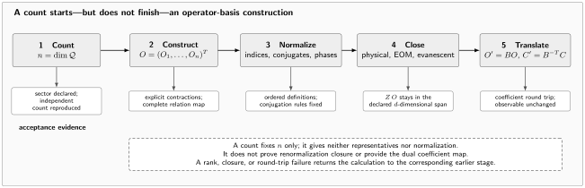
An operator-basis result is a five-stage package. Counting fixes $n=\dim\mathcal Q$; construction supplies explicit contractions and relations; normalization fixes ordering, conjugation, and phases; closure enlarges the $d$-dimensional renormalization space when EOM or evanescent operators are required; and translation applies $O'=BO$ with the dual coefficient map $C'=B^{-T}C$. The lower row states the acceptance evidence at each stage. A count alone is neither an explicit basis nor proof of RG closure. The diagram is schematic and not to scale.

Masses. For massive legs, $p_i^2=m_i^2$ rather than zero. EOM reduction can trade derivatives for masses and lower-field interactions, so homogeneous derivative grading must be replaced by a mass-refined one. Spinning massive states also carry a non-Abelian little group.

Color and other internal tensors. A color-dressed structure has the form

$$\mathcal A^{a_1\ldots a_n} =\sum_\alpha T_\alpha^{a_1\ldots a_n} \mathcal A_\alpha.$$

The $T_\alpha$ can obey finite-rank identities and transform with the kinematics under repeated-particle permutations. A single color-ordered partial amplitude is not a coordinate on the full gauge-invariant operator space.

Gauge completion. Covariant derivatives and field strengths can tie several contact multiplicities to one gauge-invariant operator. A contact list made after gauge fixing is complete only if the Ward identities and the internal invariant tensors reconstruct the same gauge-invariant class.

Dimension-specific identities and evanescents. Four-dimensional spinor-helicity variables impose four-dimensional Schouten and Gram relations. They describe the physical four-dimensional quotient, not the enlarged $d=4-2\epsilon$ counterterm space. Evanescent operators must be restored before loop renormalization, and their finite scheme map must accompany any projection back to helicity amplitudes.

Boundaries and topological terms. A total derivative has zero ordinary flat-space contact amplitude, but can carry boundary or global information. The amplitude map is not a classification of those observables.

Asymptotic-state limitations. Unstable or confined fields are not external LSZ states. Use amplitudes of stable states, gauge-invariant form factors, or an off-shell operator problem with its larger redundancy structure.

A reproducible construction test

For each amplitude basis element, retain the particle ordering, all-incoming convention, little-group weight, mass dimension, internal tensor, permutation projector, and polynomial normalization. For each operator representative, retain the exact replacement rule from momenta or spinors to derivatives and fields. The forward matrix from operator candidates to amplitude polynomials must have rank equal to the Hilbert coefficient in the identical declared sector.

A reproducible calculation compares the massless four-scalar contact count only with the four-field quotient subsector. Its required round trip is

$$\text{operator quotient} \longrightarrow \text{contact-polynomial coordinates} \longrightarrow \text{operator quotient},$$

not a map from the full scalar list containing six- and eight-field operators to four-particle amplitudes.

The operator-basis reproducibility record

For an on-shell basis, the field-content, operator-definition, basis-map, coefficient-map, and round-trip rows must contain both sides of the correspondence.

Record	Declare before reduction	Verification retained with the result
Field content and order	Spacetime dimension, dynamical fields, exact symmetries, charges, EFT grading, and truncation	Every candidate and relation has the declared labels and order
Flavor, Hermiticity, and CP	Flavor-index ranges, conjugation rule, coefficient reality conditions, and CP convention	Conjugate completion and independent real parameter count agree
Operator definition	Ordered names, explicit index contractions, derivative placement, signs, and normalization factors	Each symbolic or numerical column maps to one unambiguous operator
Renormalization data	Regulator, subtraction scheme, gauge convention when relevant, renormalization scale $\mu$, and coupling definitions	Coefficients and matrix elements use the same scheme and scale
Dimensional identities	Dimension used for Lorentz and spinor algebra, $\gamma_5$ prescription when present, and evanescent-operator definitions	The renormalized basis closes before any four-dimensional projection
Redundancy generators	IBP currents and boundary conditions, lower-order EOM, field maps, and algebraic identities	Every relation row is reproducible from a displayed generator
Basis map	Candidate and reduced dimensions, matrix orientation, exact rank, pivots, and representative ordering	Nullities and ranks satisfy the quotient dimension and no pivot is tolerance-dependent
Coefficient map	Dual transformation, transpose convention, finite shifts, and perturbative order	$C^TO$ is unchanged through the retained order
Implementation identity	Source or notebook version, dependency versions, input hash, and output checksum	A clean rerun reproduces the ordered map and checksum
Round trip and physics	Forward and inverse maps on the common subspace plus one amplitude, correlator, or counting benchmark	The round trip is the identity and the benchmark is basis independent to the stated tolerance

For the scalar application, retain $s,t,u$, the ideal $(p_i^2,\sum_i p_i,e_1)$, the $S_4$ projection, the ordered operators $(O_A,O_B,O_C)$, $R$, $c_{\rm red}$, and the amplitude normalization $\mathcal A[O_A]=2(s^2+t^2+u^2)$.

Common pitfalls

Including exchange poles in a contact basis. A pole is factorization data, not a new local polynomial. Subtract the amplitude reconstructed from lower-point vertices before reading a contact coefficient.

Comparing different field multiplicities. The full dimension-eight count includes $\phi^8$; the four-particle contact count does not.

Dropping internal tensors. Kinematic polynomials and gauge or flavor contractions are a coupled permutation problem. A kinematic count alone need not equal the color-dressed operator count.

Using a four-dimensional basis inside dimensional loops. Helicity identities can hide evanescent counterterms. Renormalize in a closed $d$-dimensional space before projecting.

Forgetting normalization in the inverse map. A one-dimensional polynomial space still permits arbitrary rescaling. Preserve the vertex convention and the dual Wilson-coefficient transformation.

Exercises

Show that there is no two-derivative local contact amplitude for four identical massless scalars.

Solution

A two-derivative scalar contact is linear in Mandelstam invariants. Bose symmetry permits only a multiple of $s+t+u$, which vanishes for four massless incoming momenta. This agrees with the absence of a $u^4t^6$ term in the multigraded scalar Hilbert series.

Starting from $R$, reduce $c_AO_A+c_BO_B+c_CO_C$ and verify the amplitude coefficient.

Solution

The relations give $O_B=-O_A/2$ and $O_C=-2O_B=O_A$. Therefore

$$c_AO_A+c_BO_B+c_CO_C =\left(c_A-\frac12c_B+c_C\right)O_A.$$

Multiplying by $\mathcal A[O_A]=2(s^2+t^2+u^2)$ gives

$$\mathcal A_4 =2\left(c_A-\frac12c_B+c_C\right) (s^2+t^2+u^2)$$

before restoring the common factor $\Lambda^{-4}$.

References

• Henning, Brian, Xiaochuan Lu, Tom Melia, and Hitoshi Murayama. 2017. “Operator Bases, S-Matrices, and Their Partition Functions.” Journal of High Energy Physics 2017: 199. DOI. Open PDF.

• Li, Hao-Lin, Zhe Ren, Ming-Lei Xiao, Jiang-Hao Yu, and Yu-Hui Zheng. 2022. “Operators for Generic Effective Field Theory at Any Dimension: On-Shell Amplitude Basis Construction.” Journal of High Energy Physics 2022: 140. DOI. Open PDF.