

Dual Evolution of Operators and Wilson Coefficients
A Wilson coefficient is a coordinate in the dual space to a renormalized operator basis. If the operators rotate and rescale with , the coefficients must evolve contragrediently so that their pairing remains unchanged. With operators stored as a column and , the chapter convention forces .
This page derives that transpose, solves noncommuting scale evolution with path ordering, and verifies the registered two-interval benchmark exactly. It also shows why preserving is necessary but not sufficient to detect a jointly reversed ordering: the differential equation and composition law provide independent checks.
Required background. Operator Anomalous-Dimension Matrices fixes , its sign, and its finite-basis covariance.
Helpful background. Form Factors and Local Operator Insertions supplies process-specific matrix elements to which coefficient vectors can be paired.
The dual equation from an invariant pairing
Section titled “The dual equation from an invariant pairing”Write a renormalized effective interaction as
Any canonical powers of a heavy scale have been included in . The operator column obeys
Scale independence of the complete interaction requires
Since this must hold for every vector in the closed operator sector,
The transpose is forced by the bilinear pairing. It is not a Hermitian conjugate: complex conjugation belongs to the separate Hermitian-conjugate operators and coefficients needed to make the action real. It is also not optional when happens to be symmetric in one example. A nonsymmetric benchmark is required to test the convention.
In row form,
Some references start from this row equation and display matrices multiplying on the right. Others define or place a minus sign in the definition of . Translation begins with the scalar pairing, not with a memorized transpose.
Ordered operator and coefficient evolution
Section titled “Ordered operator and coefficient evolution”Let
The operator evolution matrix solves
Thus
with
Here places the matrix evaluated at later RG time to the left. The composition law is
The coefficient matrix solves
Differentiating the inverse transpose of gives
so uniqueness of the initial-value problem implies
This identity already contains the ordering. There is no need to guess whether to reverse a product after transposing it.
The figure displays the two rows. Read the upper row from the earlier operator to the later operator, then compare the lower row: the coefficient map is the inverse transpose of the complete ordered product, not the transpose of each generator with the operator sign left unchanged.
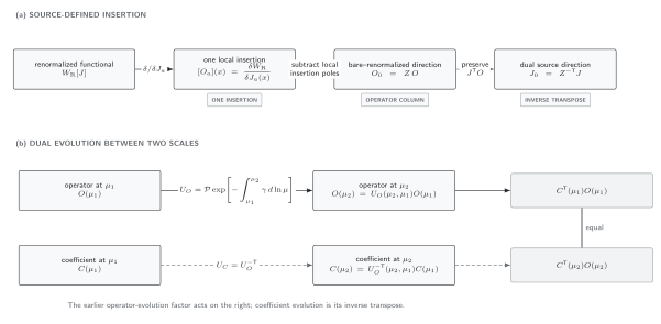
For a column operator basis, and . The equality of holds for noncommuting scale evolution as well as for a constant matrix. The original diagram is schematic and not to scale.
Exact noncommuting two-interval benchmark
Section titled “Exact noncommuting two-interval benchmark”Use the registered RG time and piecewise constant matrices
They do not commute:
For the first interval, , hence
For the second interval, , hence
The earlier factor acts on the initial column first and therefore appears on the right:
Numerically,
and
The coefficient matrix is
Choose deterministic initial data
Evolution gives
Their pairing is
at the displayed precision. The analytic value is exactly one.
Adversarial ordering and transpose checks
Section titled “Adversarial ordering and transpose checks”The same initial data expose common mistakes:
| Evolution attempted | Final pairing | Diagnosis |
|---|---|---|
| Correct , | Invariant pairing and differential equations both pass. | |
| Missing transpose: | The coefficient vector was treated as an operator coordinate. | |
| Same matrix: | Both sign and dual representation are wrong. | |
| Reversed operator product with the intended | Chronological ordering is reversed. |
If both the operator product and coefficient inverse transpose are reversed together, the scalar pairing remains invariant. That joint mistake is caught by a second test:
Equivalently, substitute the proposed into on each interval and test continuity at . Pairing invariance alone checks duality, not whether the intended time-ordered initial-value problem was solved.
A reproducible calculation uses this exact benchmark. Its accepted implementation must preserve the pairing to relative tolerance and must reject the missing-transpose and reversed-order adversarial cases.
Basis changes along the flow
Section titled “Basis changes along the flow”Let a finite, possibly scale-dependent change be
Preserving the interaction fixes
The operator anomalous dimension transforms as
Differentiating gives
only when both the inverse transpose and the derivative term are retained. At the level of finite evolution,
and therefore
The endpoint matrices matter. Applying only at one scale changes the coordinate system at one end of the evolution and is not a basis round trip.
For a constant triangular map
the induced coefficient map is
The mixing convention record requires this exact operator/coefficient round trip before a basis translation is accepted.
Matching, running, and matrix elements
Section titled “Matching, running, and matrix elements”Suppose a more microscopic theory fixes a coefficient vector at a hard scale :
Running to a lower scale gives
The low-scale amplitude is
The matrix element evolves with , so the arbitrary intermediate scale cancels when matching, running, and matrix elements use the same scheme and basis. Manohar illustrates how matrix anomalous dimensions generate operator mixing and resum leading logarithms in Wilson coefficients Manohar 2018, § 5.10.1, pp. 46–48.
At finite perturbative order, the cancellation is only accurate through the retained order. Varying probes omitted logarithmic terms, but it is not a complete uncertainty distribution. A valid scale-variation study also varies matching and matrix-element inputs coherently and does not cross a threshold without the required matching step.
Common pitfalls
Section titled “Common pitfalls”Using the operator equation for coefficients. belongs to the dual space. The transpose and opposite sign relative to follow from .
Transposing each exponential without inverting. The correct finite coefficient map is . A transpose alone does not cancel operator evolution.
Writing an unordered exponential for a running matrix. If , the ordinary exponential of the integral does not solve the initial-value problem.
Checking only the invariant pairing. Reversing both operator and coefficient products consistently can preserve the pairing while solving the wrong ordered equation. Also test the differential residual or a known composition benchmark.
Applying a basis map at only one endpoint. A scale-dependent basis change modifies and both endpoints of the evolution matrix.
Exercises
Section titled “Exercises”- Starting from and , derive the coefficient equation with indices.
Solution
Write the pairing as . Then
Relabel in the second term:
Independence of the basis operators gives , or .
- Prove directly from the operator differential equation.
Solution
From ,
Transposition gives
The initial value is the identity, so this is exactly the coefficient evolution matrix.
- Explain why when .
Solution
Use
After transposition,
Thus the later coefficient factor is also on the left. Attempting to reverse the final displayed product a second time double-counts the reversal already contained in inversion and transposition.
- Show that a simultaneous but reversed evolution can preserve and state an independent rejection test.
Solution
For any invertible trial matrix , the pair
obeys . Therefore choosing instead of passes the pairing test. It fails , the declared composition law, and the exact benchmark matrix.
Continue to Symmetry-Protected Operators, Currents, and Improvement to identify operator directions whose evolution is fixed by exact identities. Continue to Nonperturbative Renormalization Schemes and Step Scaling to replace infinitesimal perturbative running by continuum-extrapolated finite scale steps.
References
Section titled “References”-
Collins, John C. 1984; open-access reissue 2023. Renormalization: An Introduction to Renormalization, the Renormalization Group and the Operator-Product Expansion. Cambridge Monographs on Mathematical Physics. Cambridge University Press. DOI and Open PDF.
-
Manohar, Aneesh V. 2018. “Introduction to Effective Field Theories.” Lectures at the 2017 Les Houches Summer School on Effective Field Theories. arXiv:1804.05863.