

Large Logarithms and RG Improvement
Perturbation theory can fail even when every coupling is small. If a process contains separated scales, loop coefficients contain logarithms such as or . Terms of the form are no longer ordered by powers of when . Renormalization-group improvement restores a useful ordering by evaluating boundary data where its logarithms are small and transporting that data along RG characteristics.
The method has two independent accuracy labels. Logarithmic accuracy states which towers of are summed. Fixed-order matching accuracy states how many nonlogarithmic boundary coefficients are known. A complete result must declare both, together with the beta functions, anomalous dimensions, scale choices, scheme, and the interval over which the running remains perturbative.
Required background. Scale Independence and the Callan–Symanzik Equation derives the characteristic equation and the proper-vertex field sign. Beta Functions, Running Masses, and Field Anomalous Dimensions supplies the RG functions.
Helpful background. Asymptotic Scales, Remainders, Uniformity, and Optimal Truncation separates asymptotic control from convergence. Running Couplings and Dimensional Transmutation gives the one-coupling solution, and Scheme Transformations and RG Invariants explains how finite boundary terms transform.
When logarithms alter power counting
Section titled “When logarithms alter power counting”A dimensionally regulated one-loop integral with a nonexceptional Euclidean momentum has the schematic form
Subtraction removes the pole but leaves the scale logarithm. At higher orders, nested UV subtractions and repeated scale evolution generate powers of that logarithm. For a coupling whose beta function begins at , a single-logarithmic series has the form
Ordinary fixed-order counting requires both
If but , then all terms are comparable. These are the leading logarithms (LL). At the same perturbative order, are next-to-leading logarithms (NLL), followed by lower powers of .
Choosing removes the large logarithm from a single-scale boundary calculation. It does not erase the information: a coupling supplied at a remote reference scale must first be evolved to . Collins gives this large-momentum strategy and its massless-limit qualifications in Collins 1984/2023, § 7.4, pp. 185–187.
Scalar four-point logarithms
Section titled “Scalar four-point logarithms”Consider massless real scalar theory with interaction . At a nonexceptional Euclidean symmetric point, strip the overall proper-vertex sign and normalize the scalar coefficient so that its tree term is . Write
The field anomalous dimension begins at two loops in this model. With , the proper-vertex RG equation is
At the boundary , let
The constants depend on the subtraction scheme and the precise symmetric-point projection. Substituting a polynomial ansatz into the RG equation gives
Three facts are visible without evaluating a new three-loop diagram:
- the one-loop beta coefficient fixes the first logarithm ;
- repeated one-loop running fixes the LL coefficient ;
- the NLL coefficient at order combines the two-loop beta function, the one-loop boundary constant, and the first field anomalous dimension.
The explicit one-loop vertex has
equivalently . The coefficient agrees with the fixed-bare derivation of the scalar beta function in Intriligator 2007, lecture 15, pp. 1–2, PDF.
The LL recursion
Section titled “The LL recursion”Write the LL part as
Keeping only in the RG equation gives
so and
This is precisely the one-loop running coupling evaluated at :
Re-expanding the denominator reproduces every . Keeping it unexpanded is useful only while the entire characteristic remains in the perturbative domain. The formal positive-beta Landau scale is a stopping estimate, not a point through which the resummation may be continued.
Characteristic evolution and NLL structure
Section titled “Characteristic evolution and NLL structure”Let be the input coupling and let solve
from to . For the renormalized 1PI four-point coefficient, define
The characteristic solution with its boundary chosen at is
For NLL accuracy in this scalar example, use the two-loop beta function, the first nonzero , and the one-loop boundary:
Expanding this expression through returns
where . This re-expansion is the essential check that the evolution, field factor, and boundary convention have been combined with consistent signs.
Panels (a) and (b) show forward transport with increasing . The scalar vertex calculation above instead transports the boundary at back to . The dashed return arrow denotes a re-expansion check, not that inverse transport.
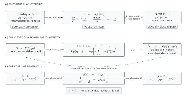
For a scalar four-point proper vertex, makes the figure’s forward exponent positive. The calculation above uses the inverse factor to transport the boundary at to ; re-expansion checks its fixed-order logarithms. Panel (c) is a distinct asymptotically free one-coupling example, not the positive-beta scalar trajectory. The diagram is schematic and not to scale.
| Figure step | Scalar four-point realization | Check |
|---|---|---|
| Boundary data | no large at | |
| Coupling evolution | one-loop solution generates | |
| Field transport | first contribution is | |
| Re-expansion | expand in | recover at order |
Declaring logarithmic accuracy
Section titled “Declaring logarithmic accuracy”For this single-logarithmic scalar vertex, the ingredients organize as follows:
| Accuracy | Towers retained | Running and transport | Boundary data |
|---|---|---|---|
| LL | ; no field factor is needed because starts at | tree term | |
| NLL | LL plus | and | one-loop constant |
| NNLL | LL, NLL, and | through and the next anomalous-dimension coefficient | through the two-loop constant |
This table is not a universal naming convention for every problem. If an anomalous dimension starts one order earlier, or if each loop produces two logarithms as in a Sudakov problem, the ingredient table and the meaning of LL change. State the tower explicitly rather than relying on the label alone.
Also distinguish a resummation label from a fixed-order label. “NLL+NLO” means that NLL towers are summed and the result is matched to the complete next-to-leading fixed-order calculation. NLL by itself does not promise every nonlogarithmic NLO contribution.
Boundary scales and matching without double counting
Section titled “Boundary scales and matching without double counting”The natural boundary scale need only be of order . Introduce
and write
The boundary function contains only , which remains moderate for an order-one variation. At all orders the dependence cancels between and . At finite order, the residual begins beyond the retained logarithmic and boundary accuracy if all ingredients are consistent.
When both a resummed prediction and a full fixed-order calculation are available, a standard additive match is
The subtraction removes the logarithmic terms present in both pieces. Re-expanding must reproduce the complete fixed-order result through the matching order. Multiplicative alternatives are possible, but they define different higher-order terms and must state their normalization and failure cases.
RG evolution never supplies missing boundary information. A finite matching constant, a new partonic channel, a threshold correction, or a power-suppressed term must be calculated or constrained separately.
Several physical scales
Section titled “Several physical scales”If an observable contains , one scale choice cannot generally make both hard and low-scale logarithms small. The remedy is a factorization or EFT statement with separately renormalized functions, schematically
The hard boundary is computed at , the low-scale boundary at , and the evolution kernel resums logarithms of . RG consistency requires the anomalous dimensions of all factors to cancel in the exact product. If rapidity as well as virtuality scales are present, an additional evolution equation is needed.
This page supplies only the general architecture. Sudakov Logarithms and Resummation develops the double-logarithmic scattering example, while Modes, Virtualities, and EFT Scale Separation begins the systematic multiscale EFT treatment. Mellin Transforms and Scaling Asymptotics provides a complementary language in which scale convolutions become products and logarithmic towers become singularity data.
Residual dependence as a diagnostic
Section titled “Residual dependence as a diagnostic”For a truncated scalar result , define the RG residual
A consistent calculation has beginning at the first omitted order. A term at an order claimed to be included identifies a missing logarithm, wrong anomalous-dimension sign, inconsistent boundary coefficient, or mismatched running input.
Useful variations probe different missing structures:
| Variation | Primarily probes | What it cannot establish by itself |
|---|---|---|
| boundary scale near its natural value | omitted logarithmic and boundary terms | a probability distribution for the error |
| matching prescription, additive versus multiplicative | formally higher-order combinations | which prescription is closer to the exact result |
| finite renormalization scheme | sensitivity to uncomputed coefficients and constants | scheme-independent uncertainty without consistent input conversion |
| threshold or factorization scales | missing matching and evolution terms | effects from absent modes or an invalid factorization theorem |
| fixed-order versus re-expanded resummation | double counting and tower reproduction | nonperturbative or power-suppressed contributions |
Vary scales only within a region where every boundary function remains free of large logarithms and the running stays controlled. A flat variation band can result from accidental cancellation, and a wide band can reflect an intentionally conservative range. Neither has a universal statistical interpretation.
Common pitfalls
Section titled “Common pitfalls”Replacing by without a boundary condition. Running transports the coupling; it does not determine . State the boundary observable or subtraction condition.
Calling a scale choice a resummation. Setting removes explicit logs from one coefficient. Resummation requires solving the evolution from the input scale and retaining the running result with a declared tower accuracy.
Using LL running with an NLO boundary and calling the result NLL. The two-loop beta function and the required anomalous dimension are part of NLL in this example. Count ingredients, not just the most accurate piece.
Double counting fixed-order logarithms. Adding fixed-order and resummed results directly repeats the expanded towers. Subtract the resummed expression through the matching order.
Searching for one scale that removes every logarithm. Multiple physical scales usually require factorization and separate boundary scales. An extreme common merely moves large logs between factors.
Evolving through a formal singularity or threshold. Stop, match to the correct degrees of freedom, or report loss of perturbative control.
Interpreting scale variation as a confidence interval. Variation is a structured stress test. It misses unknown constants, new channels, power corrections, and failures of the assumed factorization.
Exercises
Section titled “Exercises”Derive the scalar four-point coefficients through order from the RG equation.
Solution
Use
At order , the equation gives , so . At order , it gives , hence . The constant part at order gives
so .
Show that additive matching reproduces the fixed-order result through its declared order.
Solution
Let denote the expansion of the resummed result through order . Then
Applying to both sides gives
Beyond order , the unexpanded resummed towers remain.
Where to continue
Section titled “Where to continue”- Local Couplings, Trace Identities, and the Local Renormalization Group promotes couplings to sources and organizes local scale variation.
- Renormalons, OPE Ambiguities, and Power Corrections explains why perturbative reorganization still has asymptotic and power-suppressed limitations.
- Sudakov Logarithms and Resummation realizes the same boundary-plus-evolution architecture with double logarithms.
References
Section titled “References”- Collins, John C. Renormalization: An Introduction to Renormalization, the Renormalization Group, and the Operator-Product Expansion. Cambridge Monographs on Mathematical Physics. Cambridge: Cambridge University Press, 1984; open-access digital edition, 2023. DOI. Open PDF.
- Intriligator, Kenneth. “RG Equation: Beta and Gamma.” Lecture 15 outline, Physics 215B: Quantum Field Theory, University of California San Diego, 2 March 2007. PDF.