

Emergent Variables and Reorganized Effective Descriptions
New low-energy variables are justified when a gap, pole, symmetry realization, constraint, or RG attractor isolates a sector in which those variables make locality and power counting clearer. A reorganization becomes predictive only after matching observables and operators, identifying its expansion parameter, and stating where the new variables cease to span the relevant states.
The half-filled repulsive Hubbard model gives a controlled example. At , charge fluctuations are separated by an energy of order , the low-energy Hilbert space contains one spin- per site, and virtual hopping produces antiferromagnetic exchange . The spin description is emergent in a precise Wilsonian sense: its variables, interactions, and errors are derived from the electron model.
Required background. Universality Classes and Scaling Functions explains why long-distance observables can forget irrelevant microscopic details. Effective Field Theory as a Controlled Expansion supplies matching, power counting, and breakdown criteria.
Helpful background. Goldstone’s Theorem: Hypotheses and Pole Argument gives a symmetry-based route to collective low-energy fields.
A scale-separated sector licenses new variables
Section titled “A scale-separated sector licenses new variables”An effective variable is more than a renamed microscopic field. It should satisfy four tests:
- State-space test: below a stated scale, the retained variables span the states needed for the target observables.
- Matching test: microscopic operators and observables have explicit images in the reorganized theory.
- Counting test: a small parameter orders interactions and transformed observables.
- Failure test: the first omitted states, nonlocalities, or unsuppressed operators identify breakdown.
Projection, auxiliary-field transformations, quasiparticle poles, symmetry coordinates, and dual variables meet these tests in different ways. None is validated merely because it produces a compact Lagrangian.
Large U separates spin and charge
Section titled “Large U separates spin and charge”Consider the repulsive one-band Hubbard Hamiltonian
at half filling, with and . Let project onto states with exactly one electron on every site and . In the atomic limit, has energy zero after an irrelevant constant is chosen. A nearest-neighbor hop from creates a doublon–holon pair in with excitation energy .
Consequently,
There is no order- dynamics inside the half-filled low-energy sector. The first nontrivial interaction comes from two hops: one creates the virtual charge excitation and the other removes it.
The separation is controlled only when the charge gap remains large compared with the low-energy scales. At finite bandwidth this means more than writing ; the relevant comparison is with hopping-enhanced scales such as , where is a coordination number. The derivation below assumes a supplied large- regime rather than locating the Mott transition.
Degenerate perturbation theory produces superexchange
Section titled “Degenerate perturbation theory produces superexchange”A Schrieffer–Wolff transformation block-diagonalizes the Hamiltonian order by order Schrieffer and Wolff 1966, pp. 491–492. Equivalently, degenerate perturbation theory gives
Evaluating the two-hop processes on each bond yields
where
At half filling within , , so the second term is a constant. The dynamical Hamiltonian is the antiferromagnetic Heisenberg model
The sign and coefficient have a simple two-site check. Pauli exclusion blocks the virtual double occupancy for the triplet, so its shift is zero. The lower singlet eigenvalue is
The operator therefore gives exactly the leading triplet and singlet splitting, and the exact dimer displays the expected next correction.
The systematic canonical-transformation expansion and its higher-order hopping processes are derived by MacDonald, Girvin, and Yoshioka 1988, pp. 9753–9756. On a general lattice the omitted Hamiltonian terms are ; when odd virtual cycles are absent, the first corrections begin at and include longer-range and ring exchange. The advertised error must match the lattice and hopping pattern.
Operators must be transformed with the Hamiltonian
Section titled “Operators must be transformed with the Hamiltonian”If is the block-diagonalizing unitary transformation, a microscopic observable matches to
Projecting alone misses virtual-charge corrections. Spin correlators have leading images in terms of , with calculable corrections. The low-frequency electron-addition spectral function, by contrast, changes the charge sector and cannot be represented by a spin-only operator below the charge gap. This observable-level test prevents a successful energy spectrum from being overextended to every probe.
Doping supplies a direct failure case. Empty sites then belong to the low-energy projected space, no longer vanishes, and projected hopping appears at order . The appropriate leading description is a t–J-type model, not the pure Heisenberg model. Likewise, raising the probe energy toward the charge gap requires explicit doublon–holon degrees of freedom.
Hubbard Models: Symmetries and Controlled Limits gives the developed many-body treatment, including the Mott regime, superexchange, doping, and observable diagnostics.
Different reorganizations require different checks
Section titled “Different reorganizations require different checks”The Hubbard projection illustrates one route, but “emergent variable” covers several logically distinct constructions:
- Goldstone coordinates are required by a spontaneously broken exact continuous symmetry. Their derivative interactions and possible explicit-breaking masses follow from Ward identities.
- Quasiparticles are licensed by isolated poles whose width is small compared with their excitation energy. They fail when the pole dissolves into a continuum or the lifetime is not parametrically long.
- Hubbard–Stratonovich fields begin as an exact change of integration variables. They become a controlled collective description only after a saddle-point, large-, loop, or other counting rule is supplied. Hubbard–Stratonovich Fields and Collective Channels develops this route.
- Partons and dual variables may enlarge the Hilbert space and introduce gauge redundancy. Matching requires a constraint and a demonstration that physical operators and states are reproduced. Parton Constructions and Gauge Constraints develops those tests.
- Universality variables follow from attraction toward an RG fixed point. Irrelevant microscopic couplings are suppressed, while relevant deformations, symmetry data, and normalization conditions still require matching; the underlying RG logic is developed by Wilson and Kogut 1974, §§ 1–5, pp. 75–124.
The existence of a change of variables is not yet evidence that it improves locality or counting. A nonlocal duality can still be powerful, but its observable map and domain must be given rather than inferred from terminology.
When a new description is justified
Section titled “When a new description is justified”The figure organizes the evidence needed for a reorganized description. A physical gap or threshold, a quantum symmetry, and measured poles or correlators can support the new variables. Coordinate convenience and explanatory appeal may motivate the construction, but they do not replace matching.
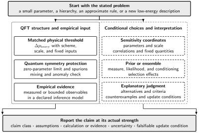
Emergent variables require structural and observable evidence: an isolated low-energy sector, symmetry or pole data, matched operators, controlled corrections, and a failure scale. Convenience, prior choice, or explanatory preference can guide a representation but cannot establish its validity. The diagram is schematic and not to scale.
A complete emergence claim records the microscopic and effective state spaces, the projection or variable map, the observables being matched, the small parameter, the first omitted operators, and the first excluded states. For the Hubbard example these are respectively electrons, singly occupied spins, the Schrieffer–Wolff map, low-energy spin observables, , higher virtual-hopping terms, and charge excitations near the Mott gap.
Emergence and naturalness answer different questions. Emergence asks which variables and interactions organize low-energy predictions. Technical naturalness asks whether small symmetry-breaking parameters remain radiatively stable. An emergent symmetry can protect coefficients, but a controlled reorganization such as the Hubbard-to-Heisenberg projection does not require a fine-tuning judgment.
Common pitfalls
Section titled “Common pitfalls”Projecting states but not observables. Use , not only , when virtual high-energy states correct the probe.
Calling every auxiliary field a particle. An exact Gaussian identity introduces a field without guaranteeing a pole or asymptotic state. Supply the spectral and power-counting checks.
Using the spin model away from half filling without modification. Holes make projected hopping an order- effect. The pure Heisenberg description then omits leading low-energy dynamics.
Quoting on an arbitrary lattice. Odd virtual cycles can generate terms. State the lattice and hopping assumptions before using the stronger remainder.
Equating universality with loss of all microscopic information. Relevant couplings, operator normalizations, symmetry realization, and matching coefficients remain necessary.
References
Section titled “References”-
MacDonald, Allan H., S. M. Girvin, and David Yoshioka. 1988. “ Expansion for the Hubbard Model.” Physical Review B 37: 9753–9756. DOI.
-
Schrieffer, J. R., and P. A. Wolff. 1966. “Relation between the Anderson and Kondo Hamiltonians.” Physical Review 149: 491–492. DOI.
-
Wilson, Kenneth G., and J. Kogut. 1974. “The Renormalization Group and the Expansion.” Physics Reports 12: 75–199. DOI.