

Loops, Counterterms, and Closure of an EFT Expansion
Loops do not invalidate an effective field theory’s operator expansion. They reveal which additional local operators are required for that expansion to close at the claimed order. The ultraviolet pole from a retained loop is absorbed by a symmetry-allowed counterterm, its logarithm drives Wilson-coefficient running, and the running cancels the explicit renormalization-scale dependence of matrix elements. This page derives those statements for a scalar EFT with one dimension-six insertion.
Required background. Power Counting and Predictive Order supplies the diagram-order formula. Operator Anomalous-Dimension Matrices fixes the operator/coefficient duality and transpose convention. Helpful background. Local Counterterms and Subdivergence Structure explains why ultraviolet subtractions are local after subdivergences are removed.
Order-by-order renormalizability
Section titled “Order-by-order renormalizability”Write a truncated EFT as
The action contains interactions of arbitrarily high canonical dimension, so it is not renormalizable with a finite number of parameters at all orders. That is not the relevant requirement. At fixed EFT order , the theory is predictive when:
- only finitely many operator classes contribute to the chosen observables;
- every ultraviolet divergence from those contributions is absorbed by operators included at order or by terms assigned systematically beyond it; and
- residual regulator and renormalization-scale dependence begins at the first omitted order.
This is order-by-order renormalizability. The counterterms are not an arbitrary repair. Locality and symmetry restrict their form, while the loop calculation fixes their divergent coefficients. Weinberg’s general EFT argument includes loop graphs generated by the most general symmetry-compatible Lagrangian, ordered so that only finitely many parameters enter any desired accuracy Weinberg 1979, pp. 331–337.
One dimension-six insertion predicts a finite counterterm sector
Section titled “One dimension-six insertion predicts a finite counterterm sector”Consider a four-dimensional massive real scalar with . The leading action contains the kinetic, mass, and terms. Add one insertion from the dimension-six generating set. For a one-particle-irreducible graph with external scalar legs, dimension-four vertices plus exactly one dimension-six vertex give superficial degree
After subdivergences are subtracted, the remaining ultraviolet pole is a local polynomial in external momenta and . The degree count and symmetry therefore predict the possible structures:
| External legs | Local dimension-six structures that can be required | |
|---|---|---|
| 0 | 6 | Vacuum terms such as |
| 2 | 4 | , , |
| 4 | 2 | , |
| 6 | 0 | |
| No new overall divergence from this one-insertion class after subdivergence subtraction |
This table is a closure envelope, not a claim that every entry has a nonzero coefficient in every diagram. Selection rules, topology, and accidental cancellations can remove mixing entries. What is unsafe is to begin with only and assume that a loop can renormalize only without checking the two- and four-point sectors.
Before reducing by integration by parts or equations of motion, a convenient generating vector is
An on-shell basis can be smaller, but then matching, renormalization, field redefinitions, and external-state restrictions must all use that same quotient. Off-shell Green functions can require EOM operators and contact terms even when an on-shell amplitude does not.
Bare and renormalized operator vectors
Section titled “Bare and renormalized operator vectors”Use the chapter convention
It follows that . For
bare independence gives the dual coefficient equation
The transpose is forced by invariance of the scalar pairing . A basis change can move entries among , anomalous dimensions, and finite coefficients, but the complete amplitude remains unchanged.
In dimensional regularization, write
where in the convention. The pole matrix records which operators mix. If a row required by the loop is absent from the chosen sector, the truncation is not closed.
Explicit logarithm and coefficient-running cancellation
Section titled “Explicit logarithm and coefficient-running cancellation”Let be the vector of tree-level matrix elements of a closed operator sector. After pole subtraction, suppose its one-loop matrix elements are
where is the logarithmic mixing matrix and is a finite matrix in the declared scheme. Then
The physical contribution is
Scale independence through requires
Indeed,
The cancellation fixes the sign and transpose independently of memory. It also states the residual honestly: an calculation is not exactly scale independent; its remaining derivative is of order plus higher EFT orders.
For one operator, the same check reads
with
Solving between and to retained order,
and substituting into removes the . This is the elementary matching-and-running consistency test reused in the next chapter.
Closure is an order lattice
Section titled “Closure is an order lattice”The figure shows two distinct ways loops enter an EFT. In the ordinary perturbative case, each retained column contains its trees or insertions, loops, and counterterms. In the shallow-scale case, a diagnosed enhancement promotes an infinite subset to leading order, after which subleading corrections and counterterms are still organized perturbatively.
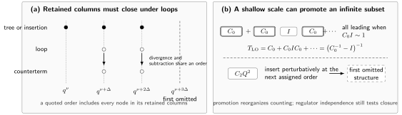
Predictive order requires closure. Panel (a) shows generic orders ; each retained column must include every tree or insertion, loop, and local counterterm assigned to it, while the dashed column is the first omitted order. Panel (b) shows the distinct case , where a shallow scale promotes the entire iteration to leading order and higher-derivative structures remain perturbative. The diagram is schematic: and the relative order of are theory dependent.
The visual rule is deliberately generic. In a derivative or chiral counting, a loop can raise the order by two powers. In a weak-coupling expansion it may instead add a factor . In a nonrelativistic threshold problem, the loop measure and propagators can promote a bubble. The increment must be derived for the modes and kinematics at hand.
Matching and running must use the same truncation
Section titled “Matching and running must use the same truncation”Suppose a Wilson coefficient is matched at a hard scale through one loop and then evolved to . A consistent prediction combines:
- the coefficient through the declared matching order;
- anomalous dimensions through the order needed to evolve that coefficient;
- EFT matrix elements through the same overall power counting; and
- threshold changes in the active operator sector.
Running cannot manufacture a finite matching constant that was never calculated, and matching at cannot replace the logarithms generated by light modes between and . Conversely, adding a threshold contribution both in and again as an EFT loop double counts it.
A reproducible calculation uses a supplied one-loop hard/infrared record to test exact infrared-pole cancellation and retained-order cancellation. The loop calculation here supplies the local closure logic behind that test.
A common uncertainty and validation checklist
Section titled “A common uncertainty and validation checklist”Loop variation is only one diagnostic, so the full record remains broader.
| Component | Record explicitly | Diagnostic or failure trigger |
|---|---|---|
| Domain and expansion parameters | Observable, kinematic window, , hard scales, thresholds, and correlations among small parameters | A threshold enters, some , or the assumed relation among parameters fails |
| Retained order and inventory | Highest order , every tree, loop, insertion, counterterm, and parameter correction included | An omitted contribution has the same assigned order as a retained one |
| Coefficient assumptions | Operator normalization, scheme and scale, expected coefficient sizes, symmetry suppressions, and any priors | Coefficients drift with fit window or require unexplained enhancement |
| EFT truncation | First omitted powers, reference size, correlation model across energies and observables, and interval interpretation | Residuals do not scale with the predicted powers or coverage fails on withheld data |
| Input and fit uncertainty | Experimental or synthetic inputs, covariance, fitted combinations, and propagation method | Results are unstable under admissible input or fit-window changes |
| Numerical uncertainty | Solver, discretization, integration, rounding, convergence tolerance, and reproducibility data | Numerical changes are not parametrically below the claimed EFT error |
| Matching and running | Matching order and scale, anomalous dimensions, threshold sequence, and residual dependence | Scale cancellation fails through the retained order or a threshold is double counted |
| Regulator, basis, and scheme checks | Regulator range, required counterterms, field/basis map, and scheme transformation | Predictions depend on an auxiliary choice at or below the claimed order |
| Model discrepancy and breakdown | Effects not represented by the EFT, validation observables, stopping rule, and alternative field content | Persistent structured residuals, new nonanalyticity, or failure across observables |
Scale variation probes some missing logarithmic terms. It does not automatically sample new operator structures, unknown finite matching constants, input errors, or model discrepancy. A narrow scale band can coexist with a large omitted power correction.
A closure check
Section titled “A closure check”For each retained loop calculation, perform these checks in order.
- Power count the integrand by regions or modes. Confirm the loop has the assigned homogeneous scaling.
- Subtract subdivergences. Only then interpret the remaining overall pole as a local counterterm requirement.
- Project onto the declared operator sector. Include EOM, total-derivative, gauge-variant, or evanescent sectors when the chosen off-shell or dimensional calculation requires them.
- Derive the coefficient RGE. Fix sign and transpose from invariance of .
- Differentiate the retained amplitude. Verify that explicit and implicit dependence cancels to the claimed order.
- Vary the regulator or subtraction prescription. Physical predictions may change only beyond the retained order after finite coefficient translations.
- Check residual scaling. The remaining regulator or scale dependence should decrease at the predicted next order.
Failure at step 3 means the operator list is incomplete. Failure at step 5 usually means a missing diagram, incorrect anomalous dimension, sign/transpose error, or mismatched perturbative order. Failure at step 6 can expose a counterterm that the counting assigned too late.
Common pitfalls
Section titled “Common pitfalls”Higher-dimension loops require infinitely many counterterms at the same order. They require an infinite tower over all orders, but only a finite local sector at fixed order and external content. The degree count above makes that finiteness explicit.
A scaleless loop vanishes, so there is no ultraviolet structure. In dimensional regularization, ultraviolet and infrared poles can cancel inside a scaleless integral. Matching must retain their origin or use an infrared prescription that keeps full and EFT contributions comparable.
Wilson coefficients and operators run with the same matrix. They run dually. With , invariance of fixes the transpose and sign conventions.
Small scale variation proves a small EFT error. Scale variation probes a limited subset of omitted terms. The first omitted operator and a complete uncertainty analysis remain necessary.
Exercises
Section titled “Exercises”For a scalar EFT with one dimension-eight insertion and otherwise dimension-four vertices, find the superficial degree of divergence of an -point graph.
Solution
The general formula is
With one insertion, . Overall local divergences can therefore occur through , subject to symmetry and topology. This predicts a finite dimension-eight counterterm sector at the retained insertion order.
Let . Write the coefficient RGE that cancels .
Solution
The coefficient vector must obey
Then , which cancels the explicit matrix-element derivative.