Relevant, Marginal, and Irrelevant Directions

Relevant, marginal, and irrelevant are properties of scaling eigenoperators at a specified fixed point, not permanent labels attached to Lagrangian monomials. A relevant perturbation grows under infrared coarse graining, an irrelevant one decays, and a marginal one requires nonlinear analysis. This classification determines tuning and corrections to scaling, but it must be refined for operator mixing, redundant directions, and dangerously irrelevant variables.

Required background. Fixed Points and Linearized RG Flow defines the stability matrix and the chapter convention $B V_I=-\theta_I V_I$. Helpful background. Free-Field OPE Preview motivates why local operators mix within symmetry sectors.

Scaling directions at a fixed point

Use dimensionless couplings $g^i$ and RG time

$$t=\ln\frac{k}{\Lambda_{\mathrm{UV}}}, \qquad \partial_tg^i=\beta^i(g).$$

Infrared evolution lowers $k$ and decreases $t$. Near a fixed point $g_\star$, let

$$B^i{}_j = \left. \frac{\partial\beta^i}{\partial g^j} \right|_{g_\star}, \qquad B V_I=-\theta_I V_I.$$

The coefficient of an eigenvector evolves as

$$c_I(t)=c_I(t_0)e^{-\theta_I(t-t_0)}.$$

Because $t-t_0<0$ toward the infrared,

$\theta_I$	Infrared behavior	Classification	Local consequence
$>0$	$c_I$ grows	relevant	must be tuned away to reach an IR fixed point
$<0$	$c_I$ decays	irrelevant	generates corrections to asymptotic scaling
$=0$	linear coefficient is constant	marginal at linear order	first nonzero nonlinear term decides

For a scalar eigenoperator $\mathcal O_I$ of fixed-point scaling dimension $\Delta_I$,

$$\delta S=c_I\int d^dx\,\mathcal O_I, \qquad \theta_I=d-\Delta_I.$$

At an interacting fixed point, $\Delta_I$ includes the anomalous dimension and the diagonalization of every operator that mixes in the chosen symmetry sector. Engineering dimension alone is exact only at a Gaussian fixed point. Even there, symmetry restrictions matter: an odd operator such as $\phi^3$ is absent if the theory is required to preserve $\mathbb Z_2$.

The terminology can be translated without memorizing competing signs. If $\lambda_I$ is an eigenvalue of the matrix $B$, then $\lambda_I=-\theta_I$. If a blocking step lowers the cutoff by $b>1$, the perturbation is multiplied by $b^{y_I}$ with $y_I=\theta_I$. For the leading irrelevant direction one often writes

$$\theta_{\mathrm{irr}}=-\omega, \qquad \omega>0,$$

so corrections decay as $b^{-\omega}$. The sign of “attractive” still depends on whether the flow is followed toward the UV or IR.

The scaling-field construction is developed in Wilson and Kogut 1974, §§ 11–12, pp. 152–176, while the systematic role of irrelevant fields in corrections to scaling is derived in Wegner 1972, pp. 4529–4534.

Gaussian scalar benchmark

Consider a real scalar field with $\mathbb Z_2$ symmetry at the Gaussian fixed point,

$$S = \int d^dx\left[ \frac12(\partial\phi)^2 +\frac12m^2\phi^2 +\frac{\lambda}{4!}\phi^4 +\sum_{n\geq3}\frac{c_{2n}}{(2n)!}\phi^{2n} +\cdots \right].$$

The free-field dimension is

$$\Delta_\phi=\frac{d-2}{2}.$$

Ignoring descendants and redundancies for the moment, the monomial $\phi^{2n}$ has dimension $n(d-2)$. Its coupling therefore has Gaussian RG exponent

$$\theta_{2n} =d-n(d-2) =2n-(n-1)d.$$

The first three cases are

$$\theta_{m^2}=2, \qquad \theta_{\lambda}=4-d, \qquad \theta_{\phi^6}=6-2d.$$

The mass is relevant in every dimension where this free scalar description is used. The quartic interaction is relevant for $d<4$, marginal in $d=4$, and irrelevant for $d>4$. The $\phi^6$ interaction is marginal at the Gaussian point in $d=3$ and irrelevant in $d>3$. These statements belong to the Gaussian fixed point; after the flow reaches an interacting fixed point, anomalous dimensions and mixing must be included again.

In four dimensions, the $\mathbb Z_2$-even classification begins as follows:

Perturbation	Gaussian dimension	$\theta$ in $d=4$	Linear class
$\int d^4x\,1$	$0$	$4$	relevant vacuum term
$\int d^4x\,\phi^2$	$2$	$2$	relevant
$\int d^4x\,\phi^4$	$4$	$0$	marginal
$\int d^4x\,\phi^6$	$6$	$-2$	irrelevant
$\int d^4x\,\phi^2(\partial\phi)^2$	$6$	$-2$	irrelevant before redundancy reduction

The field-independent vacuum term does not affect normalized nongravitational correlation functions, although it matters once vacuum energy couples to gravity. The kinetic coefficient is also dimension four, but an overall field normalization is a redundant coordinate unless it participates in a physical normalization condition or in mixing with other interactions. These qualifications show why a list of monomial dimensions is not yet a list of independent physical parameters.

Marginality is a nonlinear question

Suppose a marginal scaling coordinate $u$ has no linear term and its first nonzero beta-function coefficient is

$$\partial_tu=a u^2+O(u^3).$$

At this order,

$$\frac{1}{u(t)} = \frac{1}{u(t_0)}-a(t-t_0).$$

For a physical domain $u>0$, $a>0$ makes $u$ decrease as $t$ decreases: the perturbation is marginally irrelevant in the infrared. If $a<0$, it grows toward the infrared and is marginally relevant. If both signs of $u$ are allowed, the two sides can behave differently, so the domain and stability of the action must be stated.

Two familiar four-dimensional examples have opposite signs:

$$\begin{aligned} \partial_t\lambda &=\frac{3}{16\pi^2}\lambda^2+O(\lambda^3) &&\text{for one-component }\lambda\phi^4/4!,\\ \partial_tg &=-b_0g^3+O(g^5),\qquad b_0>0 &&\text{for an asymptotically free gauge theory.} \end{aligned}$$

Positive scalar $\lambda$ approaches the Gaussian point toward the IR and is marginally irrelevant there; toward the UV it grows and eventually leaves perturbation theory. A small positive asymptotically free gauge coupling instead grows toward the IR and is marginally relevant about the UV Gaussian point. The original gauge-theory sign calculation is given in Gross and Wilczek 1973, pp. 1343–1346 and Politzer 1973, pp. 1346–1349.

If every coefficient in the beta function vanishes along a physical, nonredundant direction, the deformation is exactly marginal and sweeps out a conformal manifold or line of fixed points. A vanishing one-loop coefficient is not enough: symmetry, higher loops, nonperturbative effects, and mixing can lift the apparent flat direction.

Eigenoperators are not arbitrary basis operators

The stability matrix acts on a vector space of perturbations. A convenient Lagrangian basis need not diagonalize it. If operators $\mathcal O_a$ mix, then only combinations

$$\mathcal O_I=v_I{}^a\mathcal O_a$$

that solve the fixed-point mixing problem have definite $\Delta_I$ and $\theta_I$. Labeling each basis monomial “relevant” or “irrelevant” before diagonalization can be wrong.

The two-coupling flow from the preceding page makes this visible. Its eigenvectors are

$$V_{\mathrm{rel}}=\begin{pmatrix}1\\0\end{pmatrix}, \qquad V_{\mathrm{irr}}=\begin{pmatrix}1\\3\end{pmatrix}.$$

A perturbation along the coordinate axis $\delta g=(0,1)^T$ decomposes as

$$\begin{pmatrix}0\\1\end{pmatrix} = -\frac13V_{\mathrm{rel}} +\frac13V_{\mathrm{irr}}.$$

Although the second coordinate axis may look unrelated to the relevant coupling, it contains a relevant component and eventually departs from the fixed point under infrared flow. The left eigenvectors of $B$ provide the appropriate projectors onto these components.

A second distinction is physical rather than algebraic. An infinitesimal local field redefinition $\phi\mapsto\phi+\varepsilon F[\phi]$ generates, schematically,

$$\delta S = \varepsilon\int d^dx\, F[\phi](x)\frac{\delta S}{\delta\phi(x)},$$

together with the regulated Jacobian contribution. This is a redundant perturbation: it changes coordinates on theory space without changing on-shell physics. Total derivatives and equation-of-motion relations create related redundancies. Operator Bases and Field Redefinitions develops their systematic removal; here the essential rule is that redundant eigenvectors are not counted as independent tunings. Wegner analyzes these invariant and redundant directions in Wegner 1974, pp. 2098–2105.

Dangerously irrelevant variables

An ordinary irrelevant coupling disappears from leading scaling because its renormalized value tends to zero. It is dangerously irrelevant when an observable or scaling function is singular in that limit, so setting the coupling to zero too early removes essential physics.

The quartic coupling above the scalar upper critical dimension is the standard example. For $d>4$ it has $\theta_u=4-d<0$ at the Gaussian fixed point, yet the ordered phase needs $u>0$ for stability. A uniform Landau free-energy density

$$f(M)=\frac12 rM^2+\frac14uM^4$$

has, for $r<0$,

$$M^2=-\frac{r}{u}, \qquad f(M_{\min})=-\frac{r^2}{4u}.$$

Both quantities are singular as the irrelevant variable $u$ tends to zero. The fixed point still controls the long-distance theory, but amplitudes and finite-size scaling cannot be obtained by simply substituting $u=0$. This mechanism is one reason naive hyperscaling fails above the upper critical dimension. Fisher’s systematic discussion appears in Fisher 1983, §§ 4–5, pp. 35–55.

The shared figure places this caveat beside the ordinary local geometry. Inspect panel (a) for the tuned and decaying directions, panel (b) for their competing magnitudes, and panel (c) for the distinction between an irrelevant coupling and an ignorable one.

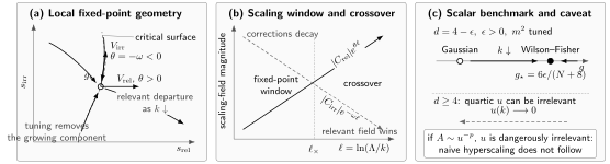
A fixed point organizes local flow, not every global trajectory. Panel (a) shows the critical surface tangent to the irrelevant eigendirection and the relevant departure under infrared flow. Panel (b) compares $e^{\theta\ell}$ growth with $e^{-\omega\ell}$ corrections for $\ell=\ln(\Lambda/k)$. Panel (c) shows the tuned one-loop $O(N)$ scalar trajectory from the Gaussian point to $g_\star=6\epsilon/(N+8)$ and the dangerously irrelevant-coupling exception to naive hyperscaling. The diagram is schematic and not to scale.

A reliable classification procedure

For an analytic or numerical RG calculation, classify perturbations in this order:

1. Specify the fixed point, spacetime dimension, symmetry sector, and RG-time orientation.
2. Form dimensionless couplings and include all operators that mix at the claimed accuracy.
3. Compute the stability operator and diagonalize it, or determine its Jordan structure.
4. Translate its eigenvalues using the declared convention; do not classify coordinate axes by inspection.
5. Analyze every zero eigenvalue at the first nonvanishing nonlinear order.
6. Remove redundant directions before counting physical relevant parameters.
7. Test whether observables are regular when irrelevant couplings are sent to their fixed-point values.
8. In a truncation, repeat the calculation under controlled basis, projection, scheme, and regulator variations.

A reproducible calculation visualizes steps 3–5 for low-dimensional flows. Critical Exponents, Scaling Relations, and Hyperscaling Caveats next explains how the physical eigenvalues enter observables.

Common pitfalls

Using engineering dimensions at an interacting fixed point. Canonical power counting supplies the Gaussian spectrum. At a non-Gaussian fixed point, anomalous dimensions and operator mixing can change both the numerical exponent and, near marginality, the classification.

Calling a coupling marginal because its linear term vanishes. Linear marginality is only a prompt to compute the first nonzero nonlinear coefficient. Exact marginality requires the beta function to vanish along a physical direction to all relevant orders.

Equating irrelevant with disposable. Irrelevant couplings govern corrections to scaling and can be dangerously irrelevant when observables are singular at their fixed-point value. They are often unnecessary as independent inputs, but not necessarily absent from controlled predictions.

Counting redundant directions as parameters. A field redefinition can generate a stability eigenvector. Parameter counting must be performed on physical theory space, after equivalent descriptions have been identified.

Exercises

1. Classify even scalar monomials

Use $\theta_{2n}=2n-(n-1)d$ to classify $\phi^2$, $\phi^4$, $\phi^6$, and $\phi^8$ at the Gaussian fixed point in $d=3,4,5$.

Solution

The exponents are

$d$	$\theta_2$	$\theta_4$	$\theta_6$	$\theta_8$
$3$	$2$	$1$	$0$	$-1$
$4$	$2$	$0$	$-2$	$-4$
$5$	$2$	$-1$	$-4$	$-7$

Positive, zero, and negative entries mean relevant, linearly marginal, and irrelevant, respectively. The $d=3$ $\phi^6$ and $d=4$ $\phi^4$ entries still require nonlinear analysis.

2. Determine marginal relevance

Let $\partial_tu=a u^2$ with $u(t_0)=u_0>0$. Find the scale at which the perturbative solution diverges and classify the two signs of $a$ under infrared flow.

Solution

The solution is

$$u(t)=\frac{u_0}{1-a u_0(t-t_0)}.$$

It has a pole at $t=t_0+1/(a u_0)$ when that value lies in the direction being followed. For $a>0$, the pole is toward the UV and $u$ decreases toward the IR, so the perturbation is marginally irrelevant in the IR. For $a<0$, the pole is toward the IR and $u$ grows there, so it is marginally relevant. The pole itself marks failure of the small-coupling approximation, not proof of a physical singularity.

3. Find the tuning hidden in a coordinate axis

For the two-coupling eigenvectors $V_{\mathrm{rel}}=(1,0)^T$ and $V_{\mathrm{irr}}=(1,3)^T$, find the condition on $(x,y)$ that removes the relevant component at linear order.

Solution

Write

$$\begin{pmatrix}x\\y\end{pmatrix} =C_{\mathrm{rel}}V_{\mathrm{rel}} +C_{\mathrm{irr}}V_{\mathrm{irr}}.$$

Then $C_{\mathrm{irr}}=y/3$ and $C_{\mathrm{rel}}=x-y/3$. The linear tuning condition is therefore

$$x=\frac{y}{3}.$$

Nonlinear terms curve the exact critical surface away from this tangent line.

4. Diagnose dangerous irrelevance

Minimize $f(M)=rM^2/2+uM^4/4$ for $r<0$, and explain why the result invalidates the substitution $u=0$ even when $u$ is RG-irrelevant.

Solution

The stationary equation is $M(r+uM^2)=0$. The stable broken minima have $M^2=-r/u$, and substitution gives $f_{\min}=-r^2/(4u)$. Both the order-parameter amplitude and the singular free energy depend on negative powers of $u$. The RG statement $u\to0$ is correct, but the observable is nonanalytic in that limit; $u$ is dangerously irrelevant.

References

• Fisher, Michael E. “Scaling, Universality and Renormalization Group Theory.” In Critical Phenomena, Lecture Notes in Physics 186, 1–139. Berlin: Springer, 1983. DOI.
• Gross, David J., and Frank Wilczek. “Ultraviolet Behavior of Non-Abelian Gauge Theories.” Physical Review Letters 30 (1973): 1343–1346. DOI.
• Politzer, H. David. “Reliable Perturbative Results for Strong Interactions?” Physical Review Letters 30 (1973): 1346–1349. DOI.
• Wegner, Franz J. “Corrections to Scaling Laws.” Physical Review B 5 (1972): 4529–4536. DOI.
• Wegner, Franz J. “Some Invariance Properties of the Renormalization Group.” Journal of Physics C: Solid State Physics 7 (1974): 2098–2108. DOI.
• Wilson, Kenneth G., and John Kogut. “The Renormalization Group and the $\epsilon$ Expansion.” Physics Reports 12 (1974): 75–200. DOI.