

Degrees of Freedom, Symmetry, and the Local Operator Expansion
An effective Lagrangian is not obtained by listing every expression of the desired canonical dimension. One must first decide which degrees of freedom propagate over the resolved scales, how exact and approximate symmetries act on them, and which local building blocks respect those actions. This page turns those decisions into an operator construction and works the first terms of a -symmetric light-scalar EFT after a heavy mediator is removed.
Required background. Effective Field Theory as a Controlled Expansion supplies the EFT domain and coefficient grammar. Multiplets, Invariants, and Selection Rules supplies representation products and invariant tensors. Helpful background. Cosets and Nonlinear Realizations develops the Goldstone and coset constructions summarized here.
Active fields are chosen by propagation, not familiarity
Section titled “Active fields are chosen by propagation, not familiarity”A degree of freedom belongs explicitly in an EFT when it can propagate over distances or times that the EFT resolves. In momentum space, this means that its pole, cut, collective excitation, or nearly on-shell region lies within the domain. A field far off shell throughout that domain can instead be eliminated and represented by local coefficients.
The decision is therefore tied to both the spectrum and the kinematics:
| Situation | Appropriate low-energy treatment |
|---|---|
| Stable particle with mass and momenta | Retain a field creating the one-particle pole |
| Goldstone boson or other gapless excitation | Retain it; its nonanalytic long-distance propagation cannot be local data |
| Heavy particle always off shell by | Remove it and expand its response in local operators |
| Narrow resonance probed near its pole | Retain a resonant field with an explicit width/pole counting |
| Shallow bound state with binding momentum | Retain or dynamically resum the pole; naive contact perturbation fails |
| Gauge potential | Retain a redundancy-compatible description when the corresponding massless or light gauge excitation is resolved |
Different EFTs can describe the same physics with different field variables. A shallow composite state may be generated by iterated contact interactions or represented by an auxiliary dimer field. These are equivalent only after coefficients, sources, and truncation rules are translated. Field names are coordinates; poles and observables decide whether the description has the needed content.
The threshold map below shows the simplest choice. The low-energy theory retains because its propagation is resolved. It removes because the chosen domain is below its pole, while preserving ’s virtual effects in local coefficients.
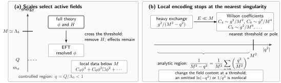
On a narrow screen, swipe the diagram or focus it and use the left/right arrow keys; Home and End move to its edges. Open the full-size diagram.
Scale separation selects the resolved states. Below the illustrative heavy scale , remains active and heavy virtual effects enter local coefficients. The dimensionless counting parameter is ; the exchanged four-momentum has mass dimension one. The heavy propagator’s geometric series converges for , while light nonanalytic propagation must remain dynamical. The diagram shows the tree-level hard contribution and is schematic, not to scale.
Symmetry data have several layers
Section titled “Symmetry data have several layers”For each proposed symmetry, record more than its group name.
- Exact or approximate: an exact symmetry forbids operators; an approximate one orders violations through explicit breaking parameters.
- Global or gauge: a global symmetry acts on physical states, while a gauge symmetry is a redundancy whose identities constrain fields, ghosts, sources, and counterterms.
- Linear or nonlinear realization: the low-energy fields may fill complete linear multiplets or realize a broken group through Goldstone transformations.
- Anomalous or nonanomalous: a quantum anomaly can obstruct gauging or require a low-energy Wess–Zumino-type term even when heavy fermions are absent.
- Internal or spacetime: spacetime symmetries constrain derivatives, indices, background structures, and sometimes the number of independent Goldstone modes.
A symmetry of the ultraviolet action need not act linearly on the retained fields. If a heavy member of a multiplet is removed, the remaining light variables can transform nonlinearly. Spontaneously broken internal symmetry provides the standard example: Goldstone fields are coordinates on a coset , and invariant interactions are constructed from covariant coset objects. Coleman, Wess, and Zumino give the general nonlinear realization and invariant-action construction in Coleman, Wess, and Zumino 1969, pp. 2239–2245, with matter fields treated by Callan, Coleman, Wess, and Zumino in Callan et al. 1969, pp. 2247–2250.
For an exact constant shift symmetry,
an undifferentiated is forbidden. The local expansion begins with derivative operators such as and higher powers of derivatives. If the shift is weakly broken, a spurion can keep the selection rule and the breaking order visible.
Spurions turn approximate symmetry into bookkeeping
Section titled “Spurions turn approximate symmetry into bookkeeping”Suppose a theory would have a symmetry except for a small parameter . Assign the formal transformation
Then the Lagrangian is built from spurion-invariant combinations. Even operators such as and can appear without , while odd operators require odd powers,
The spurion does not add a propagating particle. It records how coefficients must transform and lets the power counting include explicit symmetry suppression. Setting to its physical value at the end recovers the broken theory.
Spurions are equally useful for masses, flavor tensors, external sources, lattice anisotropies, and background fields. Their normalization must be stated: rescaling a spurion moves factors between the declared small parameter and the dimensionless coefficient.
Constructing the local operator list
Section titled “Constructing the local operator list”Given a domain and symmetry declaration, use the following sequence.
1. Fix covariant building blocks
Section titled “1. Fix covariant building blocks”List the active fields, covariant derivatives, field strengths, invariant tensors, spurions, and background structures. Record Lorentz or rotation representations, internal representations, statistics, and mass dimensions.
For a complex scalar in a gauge representation, for example, the building blocks are not arbitrary partial derivatives of but objects such as
combined into gauge-invariant scalars or into the appropriate BRST-compatible sector. Gauge fixing used in a calculation does not enlarge the physical interaction space.
2. Form spacetime and internal singlets
Section titled “2. Form spacetime and internal singlets”Contract all indices with invariant tensors, respecting Bose or Fermi statistics. Impose exact discrete symmetries, Hermiticity, and any chosen , , or classification. For an action on ordinary flat spacetime, the final local term must be a Lorentz scalar unless the EFT deliberately includes a medium velocity, boundary normal, or other spurion that breaks Lorentz symmetry.
3. Grade by all small parameters
Section titled “3. Grade by all small parameters”Attach orders for derivatives, light masses, weak couplings, spurions, loops, and field insertions according to the physical counting. Several operators of different canonical dimension can contribute at the same EFT order, and operators of the same dimension can be separated by symmetry suppression.
4. Distinguish a generating list from an independent basis
Section titled “4. Distinguish a generating list from an independent basis”At this stage the list can contain relations generated by integration by parts, equations of motion, algebraic identities, Fierz rearrangements, or field redefinitions. Those relations must be handled consistently; their systematic quotient is developed in From Operator Lists to Independent Bases. A symmetry-allowed list is not yet a proof of independence, completeness, or renormalization closure.
5. Normalize coefficients for the intended calculation
Section titled “5. Normalize coefficients for the intended calculation”State factorials, group generators, gauge couplings, loop factors, and powers of . For example,
defines different numerical coefficients from conventions that absorb or use . A quoted Wilson coefficient has meaning only together with its operator normalization and basis.
Weinberg’s prescription of using the most general local Lagrangian allowed by symmetry is powerful because it prevents ultraviolet prejudices from silently deleting low-energy interactions Weinberg 1979, pp. 327–331.
Worked example: a Z₂ light-scalar EFT
Section titled “Worked example: a Z₂ light-scalar EFT”Take the full theory
with and . Take , , real weak couplings, and . Completing the heavy-field square leaves the nonnegative terms , so the classical vacuum at the origin is stable, including the massless benchmark on the preceding page. Below , retain only . Lorentz invariance, locality, Hermiticity, and permit the schematic classes
This is a generating list, not an independent basis. Integration by parts relates derivative placements, and the leading equation of motion can trade some operators for others in on-shell observables. Keeping the unreduced list here is useful because it separates the symmetry question from the later quotient question.
The specific Gaussian heavy-mediator model generates at tree level
Together with the retained light contact term, the leading quartic is at tree level. The symmetry allows , but this Gaussian elimination generates no independent term in the displayed unreduced field variables. A later equation-of-motion reduction can move contributions into that operator. Adding an interaction, loops involving heavy fields, or other ultraviolet couplings can also change the result. The important distinction is:
Conversely, matching cannot generate a -odd operator while the full theory, regulator, vacuum, and sources preserve that symmetry. An apparent odd term would diagnose a broken assumption or inconsistent calculation.
Anomalies constrain the low-energy action
Section titled “Anomalies constrain the low-energy action”A classical symmetry can fail after quantization. If it is a gauge symmetry, an uncancelled anomaly makes the theory inconsistent rather than merely adding a suppressed operator. If it is a global symmetry, the low-energy theory must reproduce the ultraviolet anomaly even after heavy fields are removed. This may require a Wess–Zumino term whose variation accounts for the anomaly.
An anomaly is therefore neither an ordinary symmetry-breaking spurion nor evidence that all symmetry-violating operators are allowed. Its coefficient and transformation law are fixed by the anomalous Ward identity. Burgess reviews anomaly matching and its EFT implications in Burgess 2021, § 4.3, pp. 105–113.
What changes across a threshold
Section titled “What changes across a threshold”Removing a heavy field can alter the field content without changing the underlying physical symmetries. Below the threshold:
- a linear multiplet can become a nonlinear realization;
- heavy virtual effects become Wilson coefficients;
- beta functions and operator mixing change because the active loops change;
- anomaly contributions must remain represented;
- accidental low-energy symmetries can emerge because their first violation appears at high operator order; and
- a convenient operator normalization or basis can change.
The coefficient map across the threshold is a matching problem, developed in Matching, Decoupling, and Threshold Evolution. This page supplies the action space into which that matching must land.
Common pitfalls
Section titled “Common pitfalls”Every full-theory field must remain in the EFT. Fields that are uniformly far off shell can be removed. What must remain is every low-energy propagation mechanism and symmetry constraint, not every ultraviolet variable.
Every symmetry-allowed operator is equally important. Symmetry selects the allowed space; power counting ranks that space. The next page derives Power Counting and Predictive Order.
A field transforms linearly in the full theory, so it must transform linearly below the threshold. Removing partners or expanding about a symmetry-breaking vacuum can induce a nonlinear realization. The low-energy transformation law must be derived, not inherited by name.
Equations of motion may be imposed before the observable is specified. EOM relations are valid in a qualified quotient and can affect sources, contact terms, and off-shell Green functions. Integration by Parts and Equation-of-Motion Redundancy gives the full treatment.
Exercises
Section titled “Exercises”List the lowest-derivative interactions for a real Goldstone field with an exact constant shift symmetry and a separate symmetry.
Solution
Every must be differentiated because of the shift symmetry, and odd powers are forbidden by . The two-derivative kinetic term is leading. At four derivatives, examples include and terms related to before quotienting by integration by parts and equations of motion. A potential is forbidden while the shift is exact.
In a stable completion of the heavy-mediator model, include the perturbative vertex . Isolate its leading contribution and show parametrically why a interaction is generated at tree level. Additional interactions must stabilize the heavy potential; a cubic term alone does not do so.
Solution
Each of three vertices supplies , and the vertex joins the three heavy lines. At momenta small compared with , each heavy propagator contributes . Thus
up to a convention-dependent numerical factor and sign. The operator was symmetry allowed even when its coefficient vanished in the Gaussian heavy sector.
References
Section titled “References”- Burgess, C. P. Introduction to Effective Field Theory: Thinking Effectively about Hierarchies of Scale. Cambridge: Cambridge University Press, 2021. DOI
- Callan, Curtis G., Jr., Sidney Coleman, J. Wess, and Bruno Zumino. “Structure of Phenomenological Lagrangians. II.” Physical Review 177 (1969): 2247–2250. DOI
- Coleman, Sidney, J. Wess, and Bruno Zumino. “Structure of Phenomenological Lagrangians. I.” Physical Review 177 (1969): 2239–2247. DOI
- Weinberg, Steven. “Phenomenological Lagrangians.” Physica A: Statistical Mechanics and its Applications 96 (1979): 327–340. DOI