

Infrared Cancellation, Regulators, and Matching Consistency
A Wilson coefficient is short-distance data only if the full theory and EFT have identical low-energy singularities before their difference is interpreted. Infrared poles, light-mass logarithms, and soft or collinear nonanalytic terms must cancel in full minus EFT; ultraviolet poles are removed by the counterterms of the theory in which they occur. A scaleless dimensional integral does not erase this record—it can equal zero because an ultraviolet pole cancels an infrared pole.
Required background. Matching Conditions Beyond Tree Level supplies the renormalized full-minus-EFT equation. UV/IR Poles and the Renormalized-Amplitude Interface supplies pole labels, external-leg data, and amplitude conventions. Helpful background. Expansion by Regions diagnoses homogeneous loop-momentum contributions, while Soft and Collinear Singularities identifies the relevant massless pinch regions.
Infrared equality before coefficient extraction
Section titled “Infrared equality before coefficient extraction”For one projected matching object, organize the renormalized one-loop expressions as
denotes the complete infrared prescription: light masses or virtualities, dimensional or analytic regulators, contour choices, overlap subtractions, and the order in which limits are taken. The shared term can contain , , branch cuts, or distributions. It need not be small. Matching gives
so the coefficient is independent of through the retained order. The equality must hold separately for every color, spin, flavor, tensor, and operator projection being matched. A cancellation only after summing unrelated projections can hide an incomplete basis or a wrong external-state map.
In functional matching, the same statement appears as the subtraction of the EFT light-field determinant from the full light-particle-irreducible action Henning, Lu, and Murayama 2016, § 2, pp. 9–17, PDF.
The figure shows where this test sits. The common infrared term cancels in panel (b); the remaining hard term is local because all low-energy nonanalyticity has disappeared.
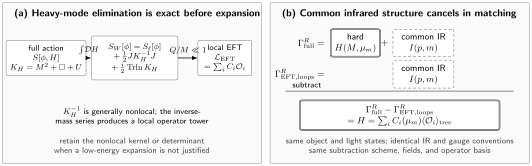
Heavy-field elimination and matching separate two steps. Panel (a) integrates a Gaussian heavy field with quadratic operator and light source , producing an exact, generally nonlocal source term and a field-dependent determinant; only for are these expanded into local operators. Panel (b) shows a renormalized loop matching condition: with the matching object, light states, infrared prescription, gauge, scheme, fields, and basis aligned, the common infrared term cancels and the remainder fixes the hard Wilson coefficients. The diagram is schematic and not to scale.
Pole algebra for an expanded amplitude
Section titled “Pole algebra for an expanded amplitude”Dimensional regularization uses one continuation parameter, , but origin labels remain essential. For the coefficient of a particular low-energy monomial, write the infrared-expanded full integral as
is removed by a full-theory counterterm. When all infrared scales have also been expanded, the corresponding EFT loop is scaleless but retains the decomposition
The EFT operator counterterm is . Consequently,
No infrared counterterm was introduced. The ultraviolet counterterms of the two theories differ, while their infrared poles agree and cancel in the matching difference. If a light mass is retained instead, the common is replaced by the same finite nonanalytic function—typically a term—on both sides. Manohar derives this pole flow and its finite-mass version in Manohar 2020, §§ 5.4–5.9, pp. 37–45, Open PDF.
A massless one-loop cancellation
Section titled “A massless one-loop cancellation”Consider the mixed light–heavy scalar integral
with and the modified-minimal-subtraction scale. Expand first in the light mass. At the term multiplying , define
The infrared-expanded full integral, after its full-theory ultraviolet subtraction, is
Expanding the heavy propagator in the EFT and then setting the light scale to zero gives
The last equality is true only after the origin labels are suppressed. Adding the EFT operator counterterm leaves
The matching difference is therefore
The massless infrared pole cancels, while the finite short-distance logarithm and constant remain. Keeping replaces the pole on each side with the same dependence and produces the identical difference. This is an independent regulator check, not a second definition of the coefficient. Burgess gives an analogous hard-plus-soft split in which an ultraviolet pole of the soft expansion cancels an infrared pole of the hard expansion in Burgess 2021, § 3.2.2, pp. 67–72.
Why a scaleless zero needs two labels
Section titled “Why a scaleless zero needs two labels”The logarithmically divergent scaleless integral obeys
One can expose the two origins by splitting the radial integral at an arbitrary nonzero scale: the large- piece supplies the ultraviolet pole and the small- piece the infrared pole; the split-scale logarithms cancel. The zero therefore means “no remaining scale after analytic continuation,” not “no ultraviolet or infrared information.”
This distinction has three consequences.
- The ultraviolet part fixes an EFT counterterm and anomalous dimension even when the unseparated loop evaluates to zero.
- The infrared part must agree with the full-theory infrared pole. Dropping it can make a correct full amplitude look inconsistent.
- Power-divergent scaleless integrals vanish without logarithmic poles in pure dimensional regularization. That fact does not remove finite heavy-threshold corrections computed from integrals that contain .
Regulators, overlaps, and orders of limits
Section titled “Regulators, overlaps, and orders of limits”Using the same infrared regulator on both sides makes cancellation visible term by term. Different regulators are permissible only if an explicit conversion demonstrates that the extracted coefficient is regulator independent. Useful choices include a small light mass, nonexceptional Euclidean virtualities, pure dimensional regularization, or an analytic regulator for a mode separation. Each choice changes intermediate expressions and may change which redundant or gauge-dependent operators are needed.
When the EFT contains several modes, its naive loop sum can count an overlap more than once. A zero-bin, overlap, or inclusion–exclusion subtraction must be specified with the mode definitions. The object compared with the full theory is then
not the uncorrected sum of region integrals. An overlap may be scaleless in one regulator and nonzero in another; its assignment still belongs in the record. Region diagnosis does not by itself define EFT fields or the subtraction prescription.
Orders of limits matter as well. Setting an external virtuality to zero before separating ultraviolet and infrared poles can turn a diagnostic integral into a scaleless zero. Taking a light mass to zero before combining degenerate real and virtual contributions can obscure an inclusive cancellation. A matching calculation should state the order of the low-energy expansion, regulator removal, on-shell limit, and threshold continuation.
Infrared and matching records
Section titled “Infrared and matching records”For each loop topology or functional trace, an infrared record should identify the full-theory term, the EFT graph and lower-order insertion that reproduces it, the regulator, the and coefficients, every light logarithm, the overlap subtraction, and the residual hard term. The scalar fixture has the minimal record:
| Item | Full theory | EFT and counterterm | Full minus EFT |
|---|---|---|---|
| Common massless singularity | 0 | ||
| EFT scaleless-loop UV part | Not an EFT graph | Removed by | |
| Hard finite term | Absent from the light loop | Matching coefficient | |
| Light-mass check | Common when | Same | Independent of |
The chapter-wide matching record below is reused unchanged on the strategy, consistency, threshold, and nondecoupling pages. Every infrared entry should point to the more detailed topology record just described.
| Record | Declare before matching | Closure check |
|---|---|---|
| Matching object and external data | Amplitude, form factor, Green function, background vertex or functional action; external species, polarizations, momenta and projections | The chosen objects span every coefficient combination claimed |
| Kinematics and retained order | On- or off-shell conditions, exceptional limits, expansion variables, inverse-mass order and loop order | Full and EFT expressions are expanded in the same variables and compared through the same order |
| Fields and normalization | Field coordinates, kinetic normalization, masses, LSZ residues and finite field maps | Two-point functions and external residues agree, or an explicit field transformation relates them |
| Gauge and auxiliary sectors | Quantum and background gauge fixing, ghosts, BRST-exact sectors and anomaly assumptions | Gauge-parameter or auxiliary-sector dependence cancels in the final observable |
| Operator basis and redundancies | Generating or reduced basis, integration-by-parts, equation-of-motion, evanescent and contact sectors | A complete map to the target basis reproduces the same amplitudes or invariant correlators |
| Ultraviolet scheme and matching scale | Regulator, subtraction convention, finite counterterms and | Scheme and dependence cancels against coefficient running and matrix elements through the retained order |
| Infrared prescription | Light masses or virtualities, infrared regulator, overlap or zero-bin subtraction and order of limits | Every common infrared pole and logarithm cancels in full minus EFT before a hard coefficient is read off |
| Threshold and decoupling assumptions | Active fields, heavy-mass origin, coupling scaling, threshold order and hierarchy among heavy scales | Sequential and one-step organizations agree to the claimed order where both are valid |
| Observable closure and uncertainty | Validation observable, input parameters, truncation estimate, numerical tolerance and fit covariance | Independent observables agree within the decomposed uncertainty and show the expected residual scaling |
A reproducible calculation can be used to vary the light regulator and matching scale. The acceptance test is that the Wilson coefficient remains stable while the full and EFT infrared terms move together.
Failure signatures
Section titled “Failure signatures”A leftover infrared pole with the correct tensor structure. The EFT loop with a lower-order operator insertion, an external-residue term, or its counterterm is often missing.
Different light logarithms. The two calculations may use different kinematics, light masses, gauge choices, or expansion orders. A Wilson coefficient cannot repair nonanalytic low-energy dependence.
A gauge-dependent hard remainder. Off-shell matching data can be gauge dependent, but a claimed physical coefficient combination or validation observable must close after field, ghost, and BRST-exact sectors are included.
Routing- or regulator-dependent mode sums. The overlap or zero-bin prescription is incomplete. Recompute the inclusion–exclusion terms before changing the hard coefficient.
A finite result obtained only by erasing labels. Setting a scaleless integral to zero before recording its UV and IR components may have cancelled poles that belong to different parts of the matching equation.
Exercises
Section titled “Exercises”Starting from the general pole decomposition, add the full and EFT counterterms and prove that the renormalized difference is .
Solution
The full counterterm is , leaving . The EFT counterterm is , leaving . Their difference is . Neither counterterm subtracts an infrared pole.
In the scalar fixture, suppose the part of the scaleless EFT integral is discarded while its UV part is retained. What failure appears?
Solution
After the EFT ultraviolet counterterm cancels the retained UV pole, the EFT side has no infrared pole. The full side still contains , so full minus EFT is infrared divergent. The failure is artificial: restoring the infrared component of the scaleless loop gives the common and cancels it.
References
Section titled “References”- Burgess, C. P. Introduction to Effective Field Theory: Thinking Effectively about Hierarchies of Scale. Cambridge: Cambridge University Press, 2021. DOI
- Henning, Brian, Xiaochuan Lu, and Hitoshi Murayama. “One-Loop Matching and Running with Covariant Derivative Expansion.” Journal of High Energy Physics 2018, no. 1 (2018): 123. DOI; arXiv
- Manohar, Aneesh V. “Introduction to Effective Field Theories.” In Effective Field Theory in Particle Physics and Cosmology: Lecture Notes of the Les Houches Summer School, Volume 108, edited by Sacha Davidson et al., 47–136. Oxford: Oxford University Press, 2020. DOI; arXiv