Scale Sensitivity and Radiative Stability

A low-energy parameter is radiatively sensitive when matching or running adds contributions that do not vanish with that parameter and are parametrically larger than its measured value. The clean diagnostic is a renormalized relation between a parent theory and its EFT, with the scheme, matching scale, and fixed inputs stated. A power divergence in a chosen regulator is neither necessary nor sufficient.

This page computes a one-loop heavy-scalar threshold, contrasts the additive $M^2$ correction to a relevant operator with the logarithmic correction to a marginal coupling, and explains what “radiative stability” does and does not mean. It does not rank ultraviolet models or turn a correction-to-parameter ratio into a probability.

Required background. Decoupling Theorems and Threshold Corrections supplies the full-to-EFT matching logic.

Helpful background. Scheme Transformations and RG Invariants separates parameter conventions from invariant predictions. EFT Truncation Errors and Breakdown Diagnostics supplies the remainder and stop-rule discipline.

Heavy thresholds make sensitivity calculable

Consider two real scalars with potential

$$V(\phi,H) = \frac{1}{2}m^2\phi^2 +\frac{1}{2}M^2H^2 +\frac{\lambda}{4}\phi^2H^2 +\frac{\lambda_\phi}{4!}\phi^4 +\cdots , \qquad M^2\gg |m^2|.$$

The light field $\phi$ is retained below $M$ and $H$ is integrated out. For a constant $\phi$ background, the heavy fluctuation has field-dependent mass

$$\mathcal M_H^2(\phi) = M^2+\frac{\lambda}{2}\phi^2.$$

In the $\overline{\mathrm{MS}}$ scheme, one real scalar contributes the one-loop effective potential

$$\Delta V_H(\phi) = \frac{\mathcal M_H^4(\phi)}{64\pi^2} \left[ \ln\!\left( \frac{\mathcal M_H^2(\phi)}{\mu^2} \right) -\frac{3}{2} \right].$$

This is the scalar specialization of the one-loop effective-potential construction Coleman and Weinberg 1973, pp. 1888–1910. Expanding for $\lambda\phi^2\ll M^2$ gives

$$\begin{aligned} \Delta V_H(\phi) ={}&\text{constant} +\frac{\lambda M^2}{64\pi^2} \left[ \ln\!\left(\frac{M^2}{\mu^2}\right)-1 \right]\phi^2 \\ &+\frac{\lambda^2}{256\pi^2} \ln\!\left(\frac{M^2}{\mu^2}\right)\phi^4 +O\!\left(\frac{\lambda^3\phi^6}{M^2}\right). \end{aligned}$$

Matching coefficients at one loop therefore yields

$$m_<^2(\mu) = m_>^2(\mu) +\frac{\lambda M^2}{32\pi^2} \left[ \ln\!\left(\frac{M^2}{\mu^2}\right)-1 \right] +O(\lambda^2),$$ $$\lambda_{\phi,<}(\mu) = \lambda_{\phi,>}(\mu) +\frac{3\lambda^2}{32\pi^2} \ln\!\left(\frac{M^2}{\mu^2}\right) +O(\lambda^3).$$

The subscripts $>$ and $<$ denote parameters just above and below the heavy threshold in the declared scheme. At the natural matching scale $\mu=M$, large logarithms vanish but the mass relation retains the finite correction

$$\Delta m_{\mathrm{th}}^2(M) = -\frac{\lambda M^2}{32\pi^2}.$$

The sign and constant term move under a finite renormalization, accompanied by a compensating change in $m_>^2$. The following structural contrast does not: the relevant operator $\phi^2$ can receive an additive contribution proportional to the physical heavy mass squared, while the dimensionless quartic receives a logarithmic correction and higher-dimension operators are suppressed by inverse powers of $M$. Matching at $\mu\sim M$ and then running in the low-energy theory keeps threshold constants separate from large logarithms Manohar 2018, §§ 2.5–2.8, preprint pp. 7–11, Open PDF.

This is not a failure of decoupling. Once $m_<^2$ is fixed by a low-energy measurement, amplitudes at $E\ll M$ have ordinary powers of $E/M$ and no experiment at fixed low-energy inputs can reconstruct $m_>^2$ uniquely. The sensitivity concerns the relation between low- and high-energy parameters under a specified matching hypothesis.

A cutoff term is not the threshold

With a hard momentum cutoff, the same tadpole may contain a term proportional to $\lambda\Lambda_{\mathrm{cut}}^2$. Dimensional regularization has no such explicit quadratic term. Bare masses and counterterms differ between the two descriptions, while a pole mass or a matched low-energy amplitude agrees after renormalization.

The physically relevant question is not whether one regulator displays $\Lambda_{\mathrm{cut}}^2$. It is whether the parent theory contains an actual state or scale $M$ whose matching contribution remains when both theories are expressed in the same renormalized inputs. Craig emphasizes this distinction: a quadratic divergence inside an isolated low-energy calculation is absorbed by renormalization, while physical additional thresholds can generate finite calculable contributions to a scalar mass Craig 2022, § 5, pp. 18–21, Open PDF.

A reliable comparison follows the sequence

$$\text{parent observable} \longrightarrow \text{renormalized matching} \longrightarrow \text{EFT parameter} \longrightarrow \text{low-energy observable}.$$

Regulator dependence cancels along this chain. If a claimed hierarchy appears only in a bare parameter or disappears when the same observable is matched in another regulator, it has not yet identified physical scale sensitivity.

Additive and multiplicative corrections differ

Let $p$ be a small renormalized parameter. A correction is multiplicative when

$$\mu\frac{dp}{d\mu} = \gamma(\{g\})\,p$$

and threshold matching has the form $p_<=Z_p p_>$ up to other declared symmetry-breaking spurions. Then $p=0$ is stable: quantum corrections do not generate a nonzero value from symmetry-preserving couplings.

An additive correction has the form

$$p_< = Z_p p_> +\Delta p(\{M_a,g_a\}), \qquad \Delta p\not\longrightarrow0 \quad\text{as}\quad p_>\longrightarrow0.$$

The two-scalar mass is of this type because $\lambda M^2$ is allowed by all stated symmetries. If $|m_<^2|\ll|\Delta m_{\mathrm{th}}^2|$, reproducing the low-energy value at the stated order requires a cancellation between $m_>^2$ and the threshold term. A transparent dimensionless report is

$$R_{\mathrm{th}} = \frac{|\Delta m_{\mathrm{th}}^2|}{|m_<^2|},$$

together with the scheme, scale, perturbative order, and split between independent matching inputs. $R_{\mathrm{th}}$ is not an observable or a probability. It records the size of one calculated contribution relative to the final parameter in a declared decomposition.

For example, with $M=10~\mathrm{TeV}$, $\lambda=0.1$, and $\mu=M$,

$$|\Delta m_{\mathrm{th}}^2| \simeq 0.0317~\mathrm{TeV}^2 = (178~\mathrm{GeV})^2.$$

If $|m_<|=100~\mathrm{GeV}$, then $R_{\mathrm{th}}\simeq3.17$. Changing $\lambda$, the parent parameter correlations, or the matching convention changes the numerical diagnostic. It does not change the performed loop calculation.

The next page asks when a quantum symmetry forces the additive term to vanish. That stronger result is Technical Naturalness and Symmetry Protection, not a consequence of the word “small.”

Keep the sources of a claim separate

The figure separates QFT structure and empirical input from conditional choices. Inspect the vertical columns: a threshold calculation, a symmetry argument, and a measurement can constrain a claim, while coordinates, priors, and explanatory criteria determine different conditional statements. All six must feed a conclusion labeled at its actual strength.

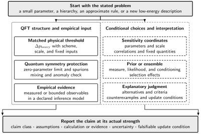
Physical thresholds, quantum symmetry protection, and measured observables supply different evidence from sensitivity coordinates, priors, and explanatory judgments. A defensible conclusion reports the claim class, assumptions, calculation or evidence, uncertainty, and a falsifiable update condition. The diagram is schematic and not to scale.

A calculated threshold does not become less real because a tuning measure is coordinate dependent. Conversely, the existence of a large threshold correction does not define a unique probability distribution over parent parameters. Keeping those statements separate allows later empirical or theoretical information to update the appropriate part of the argument.

Observable formulation and fixed inputs

The low-energy pole mass may be written schematically as

$$m_{\mathrm{pole}}^2 = m_<^2(\mu) +\Sigma_{\mathrm{light}} \bigl(m_{\mathrm{pole}}^2,\mu\bigr).$$

Its $\mu$ dependence cancels to the calculated order. A derivative such as $\partial m_{\mathrm{pole}}^2/\partial M^2$ is meaningful only after specifying what is held fixed. Holding $m_>^2(\mu)$ and $\lambda(\mu)$ fixed asks how the prediction changes along one parent-theory coordinate direction. Holding the measured pole mass fixed instead uses it as an input and merely determines how $m_>^2$ must be rematched.

This distinction prevents two common confusions:

• Input versus prediction: an observable chosen as an input cannot simultaneously be advertised as an independently predicted hierarchy.
• Independent versus correlated parameters: a UV relation $m_>^2=f(M^2)$ changes the physical trajectory and can enhance or reduce the derivative. Varying coordinates independently when the parent theory correlates them answers a different question.

Radiative stability is therefore always conditional on a theory, parameter relation, perturbative order, and observable set. It is stronger than regulator power counting and weaker than a probabilistic or explanatory conclusion.

Claim-classification table

This fixed table is used throughout the chapter. Its rows prevent a calculational result, a symmetry theorem, a sensitivity diagnostic, a probability, a measurement, and a heuristic from silently substituting for one another.

Claim class	Evidence or mathematical object	Conditional choices that must be declared	Licensed conclusion	Does not establish
Calculated threshold	Renormalized parent-to-EFT matching relation	Scheme, matching scale, matched observable, fixed inputs, and perturbative order	Size and operator structure of a heavy-scale contribution in that relation	Probability, inconsistency, or a preferred UV theory
Technical stability	Enhanced quantum symmetry, Ward identities, and spurion selection rules	Field content, symmetry limit, anomaly status, thresholds, basis, and retained order	Which corrections vanish or carry declared symmetry-breaking factors	Numerical value, typicality, or empirical success
Sensitivity diagnostic	Cancellation ratio or derivative such as $\partial\ln O/\partial\ln a_i$	Parameter coordinates, correlations, scale, observable, and quantities held fixed	Local response or cancellation in the declared chart	Coordinate-free observable, probability, or universal model ranking
Probabilistic typicality	Normalized measure, prior, likelihood, and posterior	Sample space, measure, conditioning data, selection effects, and parameterization	Probability within the declared ensemble and inference model	Ensemble-independent fact or theorem of QFT
Empirical fact	Measurement, exclusion, or reproducible bound	Dataset, likelihood, model assumptions, date, and validity domain	What observations favor or exclude within those assumptions	A unique explanatory principle or prior
Explanatory heuristic	Comparative argument about autonomy, simplicity, mechanism, or research priority	Alternatives, virtues, counterexamples, historical scope, and update conditions	A transparent conditional preference or strategy	Calculation, symmetry theorem, probability, or empirical result

The distinction between quantitative corrections, technical protection, and broader naturalness reasoning is developed from complementary perspectives by Giudice 2008, §§ 1–4, pp. 1–17, Open PDF, Craig 2022, §§ 1–2, pp. 1–7, Open PDF, and Williams 2015, §§ 2–5, pp. 84–93.

A reproducible sensitivity report

For a heavy-threshold claim, record:

1. the parent and low-energy Lagrangians, retained fields, and operator normalizations;
2. the renormalization scheme, full and EFT scales, and matching scale;
3. the physical matching object and input observables;
4. the perturbative and EFT orders;
5. the threshold relation, including its finite term and scale dependence;
6. the RG evolution above and below the threshold;
7. the independent and correlated parent parameters;
8. any correction-to-result or derivative diagnostic, labeled as conditional;
9. the first omitted order and breakdown condition; and
10. the separate empirical or explanatory conclusion, if one is made.

A cross-regulator check should reproduce the same low-energy observable after parameter conversion. A matching-scale variation should cancel against running through the calculated order. Those tests diagnose the calculation; they do not validate a prior or a research preference.

Common pitfalls

Reading a hard cutoff as a measured heavy mass. $\Lambda_{\mathrm{cut}}$ labels a regulator until a parent theory supplies a physical threshold. Match an observable before interpreting scale dependence.

Invoking decoupling to erase relevant-operator thresholds. Heavy effects in low-energy amplitudes decouple at fixed measured inputs, but relevant coefficients can receive additive powers of a physical heavy mass. These are compatible statements.

Calling the finite matching constant invariant. A finite scheme change moves constants between $m_>^2$ and $\Delta m_{\mathrm{th}}^2$. The complete matched prediction and the allowed $M^2$ structure are the appropriate comparison.

Mixing matching with running. Threshold constants are determined near $\mu\sim M$; RG evolution resums logarithms away from that scale. Combining them without double counting is part of the calculation.

Turning $R_{\mathrm{th}}$ into a probability. A correction-to-result ratio has no sample space or measure. Statistical typicality requires an explicitly normalized ensemble.

Varying parameters that a parent theory correlates. A coordinate derivative transverse to the allowed parameter surface need not describe a physical variation. State the independent inputs and their covariance or constraint equations.

Claiming technical protection before testing the quantum symmetry. A classical zero-parameter symmetry may be anomalous or broken by other couplings and thresholds. The next page performs those checks.

References

• Coleman, Sidney, and Erick Weinberg. 1973. “Radiative Corrections as the Origin of Spontaneous Symmetry Breaking.” Physical Review D 7: 1888–1910. DOI.

• Craig, Nathaniel. 2022. “Naturalness: A Snowmass White Paper.” arXiv:2205.05708 [hep-ph]. arXiv. Open PDF.

• Giudice, Gian Francesco. 2008. “Naturally Speaking: The Naturalness Criterion and Physics at the LHC.” In Perspectives on LHC Physics, edited by G. Kane and A. Pierce, 155–178. World Scientific. DOI. Open PDF.

• Manohar, Aneesh V. 2018. “Introduction to Effective Field Theories.” Les Houches lecture notes, arXiv:1804.05863 [hep-ph]. arXiv. Open PDF.

• Williams, Porter. 2015. “Naturalness, the Autonomy of Scales, and the 125 GeV Higgs.” Studies in History and Philosophy of Modern Physics 51: 82–96. DOI.