Hydrodynamic Effective-Theory Architecture

Hydrodynamics is the effective theory of disturbances whose relaxation rates vanish with frequency and wave number because they are tied to conserved quantities or other declared slow modes. Its expansion is not ordered by canonical operator dimension. One instead expands constitutive relations and, when fluctuations are retained, a doubled real-time action in $\omega\tau_{\mathrm{micro}}$ and $k\ell_{\mathrm{micro}}$ about a specified state.

For an ordinary neutral relativistic fluid, the low-energy data are the equation of state and transport coefficients; the first-order theory predicts the shear-diffusion and sound poles once those inputs are fixed. A Schwinger–Keldysh formulation adds normalization, reality, noise, and thermal KMS constraints, but hydrodynamics is selected by conserved slow variables rather than by an assumed system–environment trace.

Required background. Map the Effective-Theory Architectures supplies the common architecture card. Current Sources and Generating Functionals explains how stress tensors and currents arise from background sources.

Helpful background. Closed-Time-Path Grammar supplies the doubled real-time contour used for fluctuations and dissipation.

Conservation laws select the slow variables

Suppose the microscopic state is homogeneous on average and has a finite local equilibration time $\tau_{\mathrm{micro}}$ and correlation length $\ell_{\mathrm{micro}}$. Exact energy–momentum conservation,

$$\nabla_\mu T^{\mu\nu}=0,$$

prevents a sufficiently long-wavelength fluctuation of energy or momentum from relaxing at a nonzero rate as $k\to0$. The corresponding local densities are therefore hydrodynamic variables. A conserved $U(1)$ charge adds a density and a diffusion channel; spontaneously broken symmetries add Goldstone variables; a critical order parameter or another parametrically slow excitation must also be retained. “Fluid variables” are not a fixed particle list: they are the complete set of slow carriers in the chosen state.

For a neutral fluid away from a critical point, use a temperature field $T(x)$ and a timelike velocity $u^\mu(x)$ with $u^\mu u_\mu=1$. They parametrize the expectation value of $T^{\mu\nu}$; they are not microscopic operators with unique off-equilibrium definitions. The equation of state gives

$$p=p(T), \qquad \epsilon=\epsilon(T), \qquad w=\epsilon+p, \qquad c_s^2=\frac{dp}{d\epsilon}.$$

Here $w$ is the enthalpy density and $c_s$ is the equilibrium sound speed. These thermodynamic functions are zeroth-order matching data. Hydrodynamics does not calculate them from the conservation law.

The generating-functional viewpoint explains why the slow variables restore locality. Coupling $T^{\mu\nu}$ to a metric source makes the Ward identity a diffeomorphism identity. Integrating out the conserved-density mode would leave nonlocal response at $\omega,k\to0$; retaining a fluid map or equivalent hydrodynamic field yields a local derivative expansion. Crossley, Glorioso, and Liu construct these fields as maps between a fluid spacetime and physical spacetime and obtain the usual conservation equations as saddle-point equations Crossley, Glorioso, and Liu 2017, §§ I.B–I.D, pp. 7–19, Open PDF.

Constitutive relations carry the derivative expansion

Conservation equations are not closed until $T^{\mu\nu}$ is expressed in terms of the slow fields. Define the positive rest-space tensor

$$P^{\mu\nu}=u^\mu u^\nu-g^{\mu\nu}, \qquad P^{\mu\nu}u_\nu=0,$$

and the expansion $\theta=\nabla_\mu u^\mu$. With the site’s metric convention, define

$$\sigma^{\mu\nu} = P^{\mu\alpha}P^{\nu\beta} \left( \nabla_\alpha u_\beta+\nabla_\beta u_\alpha +\frac{2}{3}P_{\alpha\beta}\theta \right).$$

It is transverse and traceless. In the Landau frame, $u_\mu\Pi^{\mu\nu}=0$, and the parity-even neutral constitutive relation through one derivative is

$$T^{\mu\nu} = \epsilon u^\mu u^\nu +pP^{\mu\nu} +\eta\sigma^{\mu\nu} -\zeta P^{\mu\nu}\theta +O(\partial^2).$$

In the local rest frame this gives

$$T^{ij} = p\,\delta^{ij} -\eta \left( \partial_i v_j+\partial_j v_i -\frac{2}{3}\delta^{ij}\boldsymbol\nabla\!\cdot\!\mathbf v \right) -\zeta\,\delta^{ij}\boldsymbol\nabla\!\cdot\!\mathbf v +\cdots ,$$

so $\eta$ and $\zeta$ are respectively the shear and bulk viscosities. At zeroth order the equation of state is the input; at first order a neutral isotropic fluid adds these two transport functions. With a conserved charge, the chemical potential and current enter, and conductivity supplies an additional first-order coefficient. Kubo formulas or microscopic matching determine transport; symmetry and counting identify where it enters Kovtun 2012, § 1, pp. 9–16, Open PDF.

The Landau frame is a convention, not extra physics. Derivative-order redefinitions

$$T\longrightarrow T+\delta T, \qquad u^\mu\longrightarrow u^\mu+\delta u^\mu, \qquad u_\mu\delta u^\mu=0,$$

move terms among energy density, pressure, energy flow, and charge flow. They leave $T^{\mu\nu}$, conserved-current correlators, Kubo coefficients, and hydrodynamic poles unchanged to the retained order. A calculation must state its frame so that intermediate coefficients can be compared, then report frame-invariant observables.

The gradient expansion requires

$$\omega\tau_{\mathrm{micro}}\ll1, \qquad k\ell_{\mathrm{micro}}\ll1.$$

Amplitude counting is separate. Linear response assumes small departures from the reference state, while nonlinear hydrodynamics can retain order-one variation over long scales. Fluctuation loops introduce another expansion controlled by the state, spatial dimension, and coarse-graining scale; near a critical point they can require an enlarged mode set or a reorganized counting.

The hydrodynamic architecture card

Card entry	Hydrodynamic EFT choice
Degrees of freedom	Local densities tied to conserved stress tensor and currents, represented by $T$, $u^\mu$, chemical potentials, fluid maps, or equivalent fields; include every additional parametrically slow mode
Hierarchy and state	$\omega\tau_{\mathrm{micro}}\ll1$ and $k\ell_{\mathrm{micro}}\ll1$ about a declared equilibrium, stationary, or controlled nonequilibrium state
Symmetry and locality	Ward identities for conserved quantities, covariance under background gauge transformations and diffeomorphisms, and locality in a gradient expansion
Counting	Gradients, amplitudes when linearized, fluctuation or $a$-field order, and any extra critical or large-occupation parameter
Matching and inputs	Equation of state, susceptibilities, and transport from experiment, microscopic calculation, lattice methods, kinetic theory, or Kubo formulas
Outputs	Constitutive relations, hydrodynamic poles, retarded and symmetric correlators, response, noise, and long-wavelength evolution
Uncertainty	First omitted gradient and fluctuation orders, uncertainty in constitutive inputs, and sensitivity to added slow modes and state preparation
Validity boundary	A nonhydrodynamic mode is resolved, the gradient hierarchy fails, an instability changes the state, or the assumed slow-variable set is incomplete

The shared selection map places hydrodynamics on the derivative/slow-variable branch and fluctuating hydrodynamics on the doubled-state branch as well. Inspect their intersection: doubling is required for a real-time fluctuation action, but conservation—not the partial trace of a named environment—is what selects the hydrodynamic poles.

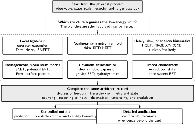
An EFT name is not a construction. Starting from the observable, state, scale hierarchy, and target accuracy, identify the dominant low-energy organizing structure, then declare degrees of freedom, symmetry and state, counting, matching or input, observables, uncertainty, and breakdown. Branches may be nested; the diagram is schematic and not to scale.

First application: shear and sound

Linearize the neutral constitutive relation about homogeneous equilibrium in flat spacetime:

$$T=T_0+\delta T, \qquad u^\mu=(1,\mathbf v)+O(v^2), \qquad w_0=\epsilon_0+p_0.$$

To first order in amplitude and gradients, energy and momentum conservation become

$$\partial_t\delta\epsilon +w_0\,\boldsymbol\nabla\!\cdot\!\mathbf v=0,$$ $$w_0\partial_t v_i +c_s^2\partial_i\delta\epsilon -\eta\nabla^2v_i -\left(\zeta+\frac{\eta}{3}\right) \partial_i(\boldsymbol\nabla\!\cdot\!\mathbf v) =0.$$

Take perturbations proportional to $e^{-i\omega t+i\mathbf k\cdot\mathbf x}$ and decompose $\mathbf v=\mathbf v_\perp+\mathbf v_\parallel$. The transverse part has $\mathbf k\cdot\mathbf v_\perp=0$, so it decouples from the energy fluctuation:

$$\left(-i\omega w_0+\eta k^2\right)\mathbf v_\perp=0.$$

Its two polarizations have the shear-diffusion pole

$$\omega_{\mathrm{shear}} = -i\frac{\eta}{w_0}k^2+O(k^4).$$

The longitudinal velocity couples to $\delta\epsilon$. Eliminating either variable gives

$$\omega^2-c_s^2k^2 +i\omega k^2 \frac{\zeta+\frac{4}{3}\eta}{w_0} =0,$$

and hence

$$\omega_\pm = \pm c_s k -\frac{i}{2} \frac{\zeta+\frac{4}{3}\eta}{w_0}k^2 +O(k^3).$$

These are the two sound poles. The same pole locations follow from the retarded stress-tensor correlators; Kovtun derives the general-$d$ attenuation coefficient and the corresponding Kubo relations Kovtun 2012, § 2, pp. 22–25, Open PDF.

For a thermodynamically stable equilibrium with $w_0>0$, $c_s^2\ge0$, $\eta\ge0$, and $\zeta\ge0$, every displayed pole lies on or below the real $\omega$ axis. At nonzero $k$, shear decays and sound attenuates. The local second law gives the same sign conditions through

$$\nabla_\mu s^\mu = \frac{\eta}{2T}\, \sigma_{\mu\nu}\sigma^{\mu\nu} +\frac{\zeta}{T}\,\theta^2 +O(\partial^3) \ge0.$$

Linear stability alone constrains the sound combination $\zeta+4\eta/3$; nonnegative entropy production separately requires the shear and bulk coefficients to be nonnegative.

This calculation is a low-$k$ test, not a causal ultraviolet completion. First-order relativistic viscous equations are parabolic and should not be extrapolated to wavelengths comparable to $\ell_{\mathrm{micro}}$. Additional relaxation variables or higher-order constitutive terms can reorganize the theory over an intermediate domain, but their coefficients and validity must be matched rather than inferred from the first-order poles.

Fluctuation constraints require a doubled contour

An ordinary constitutive theory can be written without claiming that a named environment has been traced out. To calculate fluctuations and dissipation from an action, however, one uses a closed time path:

$$Z[g_1,g_2] = \operatorname{Tr} \left( U[g_1]\,\rho_0\,U^\dagger[g_2] \right) = \int\mathcal D\chi_1\mathcal D\chi_2\, e^{iI_{\mathrm{hydro}}[\chi_1,\chi_2;g_1,g_2]}.$$

With $r$ variables denoting averages of the two legs and $a$ variables their differences, microscopic unitarity imposes the architecture-level conditions

$$I_{\mathrm{hydro}}[r,a=0]=0, \qquad I_{\mathrm{hydro}}^*[r,a] = -I_{\mathrm{hydro}}[r,-a], \qquad \operatorname{Im} I_{\mathrm{hydro}}\ge0.$$

The first expresses normalization when the two sources coincide, the second Hermiticity, and the third convergence and nonnegative noise kernels. Terms linear in $a$ impose constitutive equations at saddle level; imaginary terms quadratic in $a$ encode Gaussian noise, while higher powers describe non-Gaussian fluctuations.

For a thermal density matrix, a local KMS symmetry relates dissipative coefficients in the linear-$a$ sector to noise coefficients in the quadratic-$a$ sector. At first derivative order it reproduces fluctuation–dissipation relations, Onsager constraints when the appropriate discrete symmetry holds, and the nonnegativity of shear viscosity, bulk viscosity, and conductivity. Crossley, Glorioso, and Liu derive these relations for nonlinear fluctuating fluids and show how the standard stochastic description emerges at quadratic noise order Crossley, Glorioso, and Liu 2017, §§ I.F, III, and V.F–V.J, pp. 22–29, 44–50, and 81–88, Open PDF.

Thermal KMS is state information, not a consequence of conservation alone. A general nonequilibrium state need not obey the same local thermal symmetry, and memory or extra slow modes can spoil a local truncation. The full construction of the doubled action, nonlinear noise, and transport dynamics belongs to Schwinger–Keldysh Effective Actions for Fluids.

Hydrodynamic and open-system EFT answer different questions

Hydrodynamic EFT asks which densities remain slow because conservation laws or nearby symmetries obstruct relaxation. Open-system EFT asks what reduced dynamics follows after a chosen set of environmental variables is traced out. Either construction can use doubled fields, dissipation, and noise, but those shared tools do not make the selection criteria identical.

A closed many-body system in a mixed thermal state has hydrodynamic energy and momentum modes without an external bath. Conversely, a damped two-level system is open but has no fluid derivative expansion. Coarse-graining a fluid can produce an influence functional for its slow sector, so the two architectures can nest; when they do, the card must record both the slow-variable hierarchy and the system–environment assumptions. The next page, Open-System Effective-Theory Architecture and Consistency Conditions, isolates the latter.

Common pitfalls

Calling every long-wavelength theory hydrodynamics. Small momentum is insufficient. Hydrodynamic fields are tied to conserved quantities, Goldstones, or other parametrically slow modes whose relaxation rates vanish in the declared limit.

Treating temperature and velocity as unique operators. Away from equilibrium, derivative-order field redefinitions change their definitions and redistribute constitutive terms. State the frame and compare invariant currents, correlators, Kubo coefficients, and pole positions.

Deriving viscosities from conservation. Conservation and symmetry determine tensor structures. The equation of state and transport coefficients are matching data obtained from microscopic theory or experiment.

Using positivity of sound attenuation as the whole second law. Stable sound constrains $\zeta+4\eta/3$, whereas entropy production requires the shear and bulk channels separately to have nonnegative coefficients.

Extrapolating first-order poles to large wave number. The diffusive equation is parabolic, and the derivative truncation fails before its high-$k$ behavior can diagnose microscopic causality. A higher-order model also needs its own matched range.

Equating Schwinger–Keldysh doubling with an external bath. The closed time path computes in-in observables for closed or open systems. An open-system architecture additionally specifies a subsystem, a traced environment, an initial-state prescription, and a memory approximation.

Imposing thermal KMS on an arbitrary state. KMS encodes thermal state information. Conservation survives more generally, but fluctuation–dissipation and local thermal constraints require their stated hypotheses.

References

• Crossley, Michael, Paolo Glorioso, and Hong Liu. 2017. “Effective Field Theory of Dissipative Fluids.” Journal of High Energy Physics 2017 (9): 095. DOI. Open PDF.

• Kovtun, Pavel. 2012. “Lectures on Hydrodynamic Fluctuations in Relativistic Theories.” Journal of Physics A: Mathematical and Theoretical 45: 473001. DOI. Open PDF.