

Integration by Parts and Equation-of-Motion Redundancy
Integration by parts (IBP) and equation-of-motion (EOM) reduction are statements about a declared action and observable, not literal identities between local densities. IBP transfers derivatives and may expose a surface term. EOM operators are removed by a local perturbative field redefinition, which preserves on-shell amplitudes through the working order only after coefficients, sources, Jacobians, and induced higher-order interactions are handled consistently.
Required background. From Operator Lists to Independent Bases defines the invariant candidate space and its quotient by redundancy relations. Local versus Integrated Operator Redundancies distinguishes equality of integrated interactions from equality of local insertions. Helpful background. Boundaries, Variations, and Well-Posed Actions explains when a variational surface term vanishes and when it is physical.
Integration by parts is an action-level relation
Section titled “Integration by parts is an action-level relation”For ordinary scalar functions on a spacetime region ,
Thus and define the same bulk interaction only if the final surface integral is absent, fixed, or otherwise irrelevant to the target observable. They remain different local insertions. On a physical boundary, at a defect, or in an asymptotic sector with nonvanishing flux, the last term belongs to the problem and cannot be discarded.
IBP relations at a fixed EFT order can be generated systematically. Enumerate every local vector with one unit lower canonical dimension and the desired internal quantum numbers, take , expand it in the ordered candidate list, and row-reduce the resulting coefficient matrix. For gauge-covariant building blocks, use the covariant adjoint relation appropriate to the representation. Reordering covariant derivatives is a separate algebraic step because
produces a field-strength insertion rather than zero.
The boundary condition is part of the relation record. Saying only “drop total derivatives” silently changes the theory whenever the surface term carries charge, edge dynamics, or a source response.
Equation-of-motion operators are field-coordinate directions
Section titled “Equation-of-motion operators are field-coordinate directions”Let the EFT expansion be
where denotes a power of or another controlled small parameter. Under the local perturbative redefinition
functional Taylor expansion gives
with repeated field labels including spacetime integration. Consequently, an order- interaction proportional to can be cancelled by a redefinition with the opposite sign. This is why the leading-order EOM generates the redundancy relation at the next order.
The second line also exposes the limitation. At order , the terms involving and the second variation of are real induced interactions. Substituting a higher-order EOM into the Lagrangian does not generally reproduce them. A field redefinition is an order-by-order change of coordinates on theory space; “set the EOM to zero” is only its first-order shorthand. This distinction and its consequences for matching are derived in Criado and Pérez-Victoria 2019, §§ 2–3, pp. 5–12, and § 5.1, pp. 16–18, Open PDF.
For a path integral with sources, the same transformation changes
It also produces the functional Jacobian . For local perturbative transformations, the Jacobian can be represented by local ghost interactions and is especially simple in dimensional regularization, where the corresponding closed ghost loops vanish under the usual assumptions. That convenience is regulator- and transformation-dependent; it is not permission to omit the Jacobian without checking. Counterterms and gauge fixing must be transformed consistently as well.
Quotient domain and exceptions
Section titled “Quotient domain and exceptions”The quotient map summarizes what survives after the action-level relations are imposed. The construction of operator classes modulo IBP and EOM, including the distinction between a count and explicit representatives, is developed in Henning et al. 2016, §§ 1–2, preprint pp. 1–7, Open PDF. Read the figure’s right panel first when the target is not an ordinary on-shell scattering amplitude.
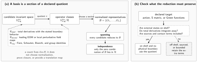
An operator basis is a normalized section of a quotient, not the unreduced candidate list or its count. Panel (a) forms classes in , chooses representatives, and tests spanning and independence separately. Panel (b) limits the reduction: on-shell observables with boundary conditions that remove total derivatives use the quotient, whereas off-shell Green functions, explicit sources and contact terms, or physical boundaries can require the extra operators. The diagram is schematic and not to scale.
The local reason for the off-shell exception is the Schwinger–Dyson identity. For any insertion and local functional ,
up to the stated path-integral convention. The right side consists of coincident-point contact terms. It vanishes in separated on-shell matrix elements after LSZ reduction under the equivalence-theorem hypotheses, but not in a general sourced Green function. Arzt proves the quantum EOM reduction while keeping precisely this on-shell/off-shell distinction in Arzt 1995, § 2, preprint pp. 4–7, Open PDF. This is the perturbative EFT realization of the field-coordinate equivalence established in Kamefuchi, O’Raifeartaigh, and Salam 1961, pp. 529–549.
The resulting decision is concrete:
- For an on-shell -matrix element with ordinary asymptotic fields and a vanishing surface term, reduce by IBP and leading EOM and transform the Wilson coefficients.
- For off-shell correlators, transform the sources and retain the induced contact terms, or work in an enlarged Green-function basis.
- For a physical boundary, retain the surface operator and specify its boundary condition or boundary coupling.
- At the next EFT order, include every interaction generated by the earlier field redefinition before reducing again.
First application: derivative scalar operators
Section titled “First application: derivative scalar operators”Return to the four-dimensional -even scalar theory, now writing the dimension-six action explicitly:
IBP gives
so define . After this action-level step, the dimension-six interaction is .
Now set
The lower-order action changes by
Choosing removes the derivative operator and leaves
This reproduces the relation-matrix result on the preceding page. The transformation of the dimension-six terms themselves starts at ; it may be omitted here because the action has been declared only through . A calculation through must retain it and add the required second-order field redefinition.
The same result can be checked without using the interacting example. Take a free massive scalar with EOM and the redundant interaction
After symmetrizing over four identical external legs, its tree-level contact vertex is proportional to
Every external leg satisfies , so the on-shell amplitude vanishes. Off shell, the same polynomial is nonzero and supplies exactly the inverse-propagator contact structure predicted by the Schwinger–Dyson identity. This is a direct observable-domain check, not merely a formal substitution.
The operator-basis reproducibility record
Section titled “The operator-basis reproducibility record”Every reduction should carry enough information for another calculation to reconstruct the same quotient and translate coefficients into or out of it. The following semantic table is the chapter-wide minimum; later pages reuse it while specializing the relevant rows.
| Record | Declare before reduction | Verification retained with the result |
|---|---|---|
| Field content and order | Spacetime dimension, dynamical fields, exact symmetries, charges, EFT grading, and truncation | Every candidate and relation has the declared labels and order |
| Flavor, Hermiticity, and CP | Flavor-index ranges, conjugation rule, coefficient reality conditions, and CP convention | Conjugate completion and independent real parameter count agree |
| Operator definition | Ordered names, explicit index contractions, derivative placement, signs, and normalization factors | Each symbolic or numerical column maps to one unambiguous operator |
| Renormalization data | Regulator, subtraction scheme, gauge convention when relevant, renormalization scale , and coupling definitions | Coefficients and matrix elements use the same scheme and scale |
| Dimensional identities | Dimension used for Lorentz and spinor algebra, prescription when present, and evanescent-operator definitions | The renormalized basis closes before any four-dimensional projection |
| Redundancy generators | IBP currents and boundary conditions, lower-order EOM, field maps, and algebraic identities | Every relation row is reproducible from a displayed generator |
| Basis map | Candidate and reduced dimensions, matrix orientation, exact rank, pivots, and representative ordering | Nullities and ranks satisfy the quotient dimension and no pivot is tolerance-dependent |
| Coefficient map | Dual transformation, transpose convention, finite shifts, and perturbative order | is unchanged through the retained order |
| Implementation identity | Source or notebook version, dependency versions, input hash, and output checksum | A clean rerun reproduces the ordered map and checksum |
| Round trip and physics | Forward and inverse maps on the common subspace plus one amplitude, correlator, or counting benchmark | The round trip is the identity and the benchmark is basis independent to the stated tolerance |
For the scalar example, the candidate dimension is , the relation rank is , and the reduced dimension is . The exact map is
Its on-shell benchmark is the vanishing four-point matrix element of above. Its failure records are equally important: nonzero boundary flux, untransformed sources, or a requested prediction blocks the naive elimination.
Common pitfalls
Section titled “Common pitfalls”Writing inside every operator. EOM replacement is a controlled field redefinition at a specific EFT order. Apply it to the higher-order sector using the lower-order action, then record the induced coefficient map.
Forgetting that IBP and derivative commutation are different. Moving a covariant derivative and swapping two covariant derivatives are separate operations; the latter can generate a field strength.
Checking only the transformed action at first order. The same transformation changes sources, counterterms, the measure, and higher-order interactions. Which pieces matter is fixed by the observable, regulator, and target accuracy.
Using an off-shell zero as an on-shell theorem. An EOM insertion equals contact terms in a Green function. It disappears from the matrix only after the complete equivalence-theorem argument.
Exercises
Section titled “Exercises”Derive the scalar coefficient shift without first integrating by parts.
Solution
Substituting directly into gives
Choose to remove . This shifts to and leaves . A second description using the IBP relation then removes and shifts by , giving the same .
Why does a single insertion of need not vanish in a two-point Green function even though it is redundant for the matrix?
Solution
The Schwinger–Dyson identity differentiates both and the inserted fields. Functional derivatives of the inserted fields produce delta-function contact terms, so the off-shell correlator changes. LSZ multiplication by inverse propagators and the consistent transformation of interpolating fields remove the redundant direction from on-shell amplitudes under the theorem’s hypotheses.
References
Section titled “References”- Arzt, Christopher. “Reduced Effective Lagrangians.” Physics Letters B 342, no. 1–4 (1995): 189–195. DOI; Open PDF
- Criado, Juan Carlos, and Manuel Pérez-Victoria. “Field Redefinitions in Effective Theories at Higher Orders.” Journal of High Energy Physics 2019, no. 3 (2019): 038. DOI; Open PDF
- Henning, Brian, Xiaochuan Lu, Tom Melia, and Hitoshi Murayama. “Hilbert Series and Operator Bases with Derivatives in Effective Field Theories.” Communications in Mathematical Physics 347, no. 2 (2016): 363–388. DOI; Open PDF
- Kamefuchi, S., L. O’Raifeartaigh, and A. Salam. “Change of Variables and Equivalence Theorems in Quantum Field Theories.” Nuclear Physics 28 (1961): 529–549. DOI