Integrating Out Heavy Fields

Integrating out a heavy field means performing its functional integral while retaining the light fields as dynamical variables. The result is an exact light-field action that is generally nonlocal. A local EFT appears only after this action is expanded in low momenta and light masses over the heavy scale. For a Gaussian heavy scalar, the calculation cleanly separates the classical source term, the heavy-field determinant, and any measure contribution.

Required background. Effective Field Theory as a Controlled Expansion supplies the inverse-scale hierarchy and target order. Scale Separation, Locality, and the Domain of an EFT identifies the analyticity domain of the local expansion. The 1PI Effective Action and Mean-Field Equations supplies the Legendre-transform and saddle-point language. Helpful background. Heat Kernels, Zeta Functions, and Spectral Determinants develops one route for evaluating local determinant coefficients.

Heavy-mode path integral and the Wilson action

Split the fields into light variables $\phi$ and a heavy real scalar $H$. The Wilson action for the light fields is defined by

$$e^{iS_W[\phi]} = \int \mathcal D H\,\mu[\phi,H]\, e^{iS[\phi,H]}.$$

Only the heavy variable is integrated here. Low-energy observables still require the remaining light-field path integral built from $S_W$. Consequently, the Wilson action is not the same object as the full light-field 1PI effective action beyond tree level: the latter also contains light loops.

For a Gaussian heavy sector, write

$$S[\phi,H] = S_\ell[\phi] -\frac12 H\mathcal K_H[\phi]H -J[\phi]H,$$

where repeated spacetime arguments are integrated and

$$\mathcal K_H[\phi] = \Box+M^2+U[\phi].$$

Completing the square with

$$H_c[\phi] = -\mathcal K_H^{-1}J$$

gives, up to a field-independent normalization,

$$\boxed{ S_W[\phi] = S_\ell[\phi] +\frac12J\mathcal K_H^{-1}J +\frac{i}{2}\operatorname{Tr}\ln\mathcal K_H +S_{\mathrm{measure}}[\phi] }.$$

The inverse and determinant inherit the contour and boundary conditions of the observable. An in–out amplitude uses the Feynman inverse; an initial-value or closed-time-path problem needs the corresponding causal contour. In Euclidean signature, one instead studies the inverse of an elliptic operator with declared boundary conditions. Writing only $1/(\Box+M^2)$ without this information does not define the nonlocal action completely.

The three nonclassical-looking terms have distinct origins.

• The source term $J\mathcal K_H^{-1}J/2$ is obtained by substituting the classical heavy-field solution and is tree level in the full theory.
• The trace logarithm is the Gaussian heavy-field fluctuation determinant. If $\mathcal K_H$ depends on $\phi$, it generates diagrams with one closed heavy loop and arbitrary light-background insertions.
• $S_{\mathrm{measure}}$ records Jacobians, gauge-fixing determinants, and ghosts when the measure is not a constant Cartesian scalar measure. A Jacobian may vanish or become a local counterterm in a particular regularization, but that is a result to establish rather than a term to omit by definition.

If the heavy action has cubic or higher powers of $H$, the displayed formula is the first part of a saddle-point expansion. Higher connected vacuum graphs of the heavy fluctuations add higher-loop terms. Burgess distinguishes this Wilson action from the low-energy 1PI generator and derives their relation in Burgess 2021, §§ 2.2–2.3, pp. 26–38.

The figure summarizes the two operations that must remain distinct. Panel (a) is the exact heavy-field integration followed by a conditional local expansion. Panel (b) previews matching: light-region contributions common to the full and effective theories cancel before the hard coefficient is identified.

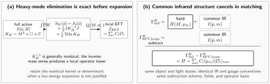
Heavy-field elimination and matching separate two steps. Panel (a) integrates a Gaussian heavy field with quadratic operator $K_H=M^2+\Box+U[\phi]$ and light source $J[\phi]$, producing an exact, generally nonlocal source term and a field-dependent determinant; only for $Q/M\ll1$ are these expanded into local operators. Panel (b) shows a renormalized loop matching condition: with the matching object, light states, infrared prescription, gauge, scheme, fields, and basis aligned, the common infrared term cancels and the remainder fixes the hard Wilson coefficients. The diagram is schematic and not to scale.

Exact elimination of the chapter’s heavy scalar

Take the light/heavy model

$$\mathcal L = \frac12(\partial\phi)^2 +\frac12(\partial H)^2 -\frac12M^2H^2 -\frac g2H\phi^2.$$

After integrating the heavy kinetic term by parts,

$$\mathcal K_H=\Box+M^2, \qquad J=\frac g2\phi^2.$$

The heavy equation of motion and its solution are

$$(\Box+M^2)H_c = -\frac g2\phi^2, \qquad H_c = -\frac g2\frac{1}{\Box+M^2}\phi^2.$$

Substitution, or equivalently completion of the functional square, yields

$$S_W[\phi] = S_\ell[\phi] +\frac{g^2}{8} \int d^4x\,d^4y\, \phi^2(x)G_H(x-y)\phi^2(y),$$

where

$$(\Box_x+M^2)G_H(x-y)=\delta^{(4)}(x-y)$$

with the selected boundary condition. This bilocal term is exact for the normalized light-field functional integral of this model. Because $\mathcal K_H$ is independent of $\phi$, its determinant is a field-independent vacuum factor and cancels from normalized light correlators. This does not mean that the low-energy theory has no loops: light-field integration over the nonlocal vertex remains.

The bilocal kernel also explains why eliminating a particle is not literally deleting its effects. The heavy pole, propagation, and crossed-channel structure remain encoded in $G_H$ until a low-energy expansion is made.

From the nonlocal kernel to local operators

For Fourier components satisfying $|q^2|<M^2$,

$$\frac{1}{M^2+\Box} = \frac1{M^2} -\frac{\Box}{M^4} +\frac{\Box^2}{M^6} +O(M^{-8}).$$

The corresponding local Lagrangian is

$$\begin{aligned} \mathcal L_{\mathrm{EFT}} =\mathcal L_\ell &+\frac{g^2}{8M^2}\phi^4 -\frac{g^2}{8M^4}\phi^2\Box\phi^2\\ &+\frac{g^2}{8M^6}\phi^2\Box^2\phi^2 +O(M^{-8}). \end{aligned}$$

Integration by parts can move derivatives among the fields, and later field redefinitions can remove equation-of-motion operators. Those transformations change the displayed coefficients and basis, not the on-shell prediction. It is therefore safest to perform the expansion in a generating basis, verify matching, and only then translate to the desired reduced basis.

The leading contact term provides a useful combinatorial check. Its four-identical-field vertex is

$$i\,4!\left(\frac{g^2}{8M^2}\right) = i\frac{3g^2}{M^2},$$

which equals the leading contribution from the $s$, $t$, and $u$ heavy-exchange channels. Through $1/M^6$, the reduced tree amplitude is

$$\frac{\mathcal A_{\mathrm{EFT}}}{g^2} = \frac3{M^2} +\frac{s+t+u}{M^4} +\frac{s^2+t^2+u^2}{M^6}.$$

This agrees term by term with

$$\frac{\mathcal A_{\mathrm{full}}}{g^2} = \frac1{M^2-s} +\frac1{M^2-t} +\frac1{M^2-u}.$$

For massless on-shell scattering, $s+t+u=0$. The vanishing amplitude correction is a kinematic cancellation; the dimension-six structures still occur in the local action and can contribute to other matrix elements. Tree-Level Matching and Classical Elimination develops the amplitude comparison and residual check in full.

When the determinant carries physics

Add a quadratic portal,

$$\Delta\mathcal L = -\frac{\kappa}{4}H^2\phi^2.$$

Then

$$\mathcal K_H[\phi] = \mathcal K_0+U[\phi], \qquad \mathcal K_0=\Box+M^2, \qquad U=\frac{\kappa}{2}\phi^2,$$

and the field-dependent part of the determinant is

$$\frac{i}{2}\operatorname{Tr}\ln(1+\mathcal K_0^{-1}U) = \frac{i}{2}\operatorname{Tr} \left[ \mathcal K_0^{-1}U -\frac12\mathcal K_0^{-1}U\mathcal K_0^{-1}U +\cdots \right].$$

The trace includes the loop momentum and spacetime integration. Its ultraviolet-divergent local terms renormalize light-theory operators; its finite hard terms supply one-loop matching coefficients. A covariant derivative or heat-kernel expansion organizes these terms when the light background varies slowly. Henning, Lu, and Murayama separate pure-heavy determinants, mixed heavy–light loops, and the nonlocal action needed to connect them in Henning, Lu, and Murayama 2016, §§ 1.1 and 2, pp. 2–17; Appendix C, pp. 53–55, PDF.

Mixed loops require particular care. Integrating over $H$ while holding $\phi$ fixed produces pure-heavy closed loops directly. Diagrams containing both heavy and light internal propagators arise after the remaining light integration over nonlocal vertices, or equivalently from a resolved functional matching formalism. Expanding a determinant and calling it the entire one-loop answer can therefore miss mixed contributions.

Locality, symmetry, and stopping conditions

The local expansion is justified when every background derivative, external invariant, and light mass entering the kernel is small compared with the nearest heavy singularity, and when this hierarchy is uniform over the field configurations in use. Keep the nonlocal action, change the degrees of freedom, or restrict the domain when:

• an invariant approaches the heavy pole or a production threshold;
• $M^2+U[\phi]$ develops a small or zero eigenvalue on the background;
• a massless or light mode was placed in the heavy determinant and generates nonanalytic low-energy behavior;
• boundary or initial-state effects make the derivative expansion nonuniform; or
• an anomalous determinant phase or topological term survives the heavy limit.

If the functional measure and regulator respect a linearly realized light-field symmetry, the Wilson action inherits it. For the scalar fixture, every induced term is even under $\phi\mapsto-\phi$. For gauge symmetries, a background-covariant calculation can keep covariance manifest, but the quantum gauge fixing, ghosts, BRST-exact sectors, and anomaly conditions still belong in the derivation. “Integrating out preserves symmetry” is true only with those qualifications.

Common pitfalls

The classical equation is the whole effective action. It gives the tree source term. A field-dependent determinant, measure Jacobian, and higher heavy loops can contribute beyond tree level.

The Wilson action is the low-energy 1PI action. The Wilson action contains the influence of modes already integrated out. Light loops must still be computed, and they are essential in loop matching.

A nonlocal kernel is an EFT failure. The exact result after eliminating a field is expected to be nonlocal. Locality is an additional low-energy expansion whose domain must be checked.

A zero on-shell correction deletes an operator. Observable-specific identities such as $s+t+u=0$ can hide an operator in one amplitude without making it redundant in the action.

Exercises

Complete the square in $-H\mathcal K_HH/2-JH$ and verify the sign of the source term in $S_W$.

Solution

Set $H=H'+H_c$ with $H_c=-\mathcal K_H^{-1}J$. Then

$$-\frac12H\mathcal K_HH-JH = -\frac12H'\mathcal K_HH' +\frac12J\mathcal K_H^{-1}J.$$

The linear term in $H'$ cancels. The remaining Gaussian integral produces the determinant, while the classical source term has the positive sign displayed.

Why does the coefficient $g^2/(8M^2)$ reproduce three exchange channels rather than one?

Solution

The local monomial contains four identical fields, so differentiating the interaction action four times gives a factor $4!=24$. Its vertex is therefore $i(24)g^2/(8M^2)=i3g^2/M^2$. The full amplitude has one leading $ig^2/M^2$ term in each of the $s$, $t$, and $u$ channels, giving the same sum.

References

• Burgess, C. P. Introduction to Effective Field Theory: Thinking Effectively about Hierarchies of Scale. Cambridge: Cambridge University Press, 2021. DOI
• Henning, Brian, Xiaochuan Lu, and Hitoshi Murayama. “One-Loop Matching and Running with Covariant Derivative Expansion.” arXiv:1604.01019 [hep-ph] (2016). arXiv