

Running and Matching across Multiple Thresholds
When a process contains separated scales , no single beta function evolves its Wilson coefficients from top to bottom. Running resums logarithms while the active fields and operator basis are fixed; matching changes that theory near each heavy mass. A consistent prediction is therefore an ordered composition of evolution, threshold, parameter, and basis maps whose dependence on the arbitrary matching scales cancels through the calculated order.
Required background. Decoupling Theorems and Threshold Corrections explains why mass-independent schemes require explicit thresholds. Large Logarithms and RG Improvement supplies the resummation logic, and Anomalous Dimensions and Wilson-Coefficient Evolution supplies coefficient-space evolution. Helpful background. Multiple Couplings and Coupled RG Flows develops the simultaneous running of the parameters entering the matrices below.
The ordered coefficient map
Section titled “The ordered coefficient map”Call the theories above , between and , and below the high, intermediate, and low EFTs. In any one interval, collect the coefficients into a column and define the coefficient-space anomalous dimension by
Its evolution operator is
with . The path ordering matters when anomalous-dimension matrices at different scales do not commute.
At a threshold , the most general linear matching relation needed at a fixed EFT order is affine:
The matrix transfers coefficients already present above the threshold. The vector accounts for operators or lower-dimensional parameter shifts generated even when the corresponding high-scale Wilson coefficients vanish. It can be absorbed into a homogeneous matrix by augmenting with the running parameters and a constant component.
For two thresholds, the three stages are
Thus the order of operations is fixed by scale. In particular, and cannot generally be multiplied as if they acted on the same vector space: the intermediate evolution and any finite basis translation belong between them. The classic weak-decay construction gives this same step-by-step structure, including flavor-dependent evolution and threshold matrices, in Buchalla, Buras, and Lautenbacher 1996, §§ III.D.1–2 and III.F.2, pp. 26–29 and 34–35, Open PDF.
The figure makes the composition and its domain test explicit. Read the left panel downward: each horizontal crossing changes the theory, while each vertical segment runs within one theory.
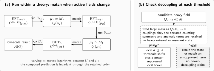
Sequential threshold evolution is an alternation, not one continuous beta function. Panel (a) evolves coefficients with , matches with near , evolves with , matches with near , and finally evolves to the observable scale; dependence on the arbitrary matching scales cancels through the retained order. Panel (b) checks the hierarchy, heavy-mass limit, coupling counting, symmetry and anomaly terms, and external kinematics. Passing gives shifts of operators with dimension at most four plus an inverse-mass-suppressed local tower; failure requires retaining the state or matching an unsuppressed effect. The diagram is schematic and not to scale.
Matching-scale cancellation
Section titled “Matching-scale cancellation”The matching points are organizational choices, not physical scales. For a homogeneous threshold relation, differentiating with respect to its matching point gives the consistency equation
where is the total derivative: it acts on the explicit dependence and on every running coupling, mass, and gauge parameter inside . This equation says that moving the threshold is compensated by the different evolution above and below it. The augmented coefficient vector gives the corresponding equation for an affine map.
At all orders, inserting this relation into the ordered chain gives
after all inputs are transported consistently. At finite order the derivative begins at the first omitted matching or running order. A residual at an order that was supposedly retained instead diagnoses a missing threshold logarithm, an inconsistent anomalous dimension, or a parameter that was not converted between the two theories. The cancellation of matching-scale and scheme dependence through the working order is exhibited explicitly in Buchalla, Buras, and Lautenbacher 1996, § III.F.4, pp. 39–40, Open PDF.
Basis and scheme translations
Section titled “Basis and scheme translations”Thresholds can change the number and definition of operators. Let the Lagrangian interaction be , with a column of operators. If a finite basis change is
then invariance of requires
Consequently, evolution and matching matrices transform as
These relations are more than notation. A reduced on-shell basis, a Green-function basis containing equation-of-motion operators, and a dimensional-regularization basis containing evanescent operators can have different dimensions and finite counterterms. Then may be rectangular, and the finite projection must be included at the threshold. Couplings, masses, field normalizations, gauge conventions, and the evanescent prescription must also be translated before a matrix from one interval is combined with the next. Wilson coefficients may jump; matched observables do not.
First application: two separated thresholds
Section titled “First application: two separated thresholds”Consider one coefficient with no additive source. To isolate the composition, take constant coefficient anomalous dimensions
so . Use common arbitrary units with
and set , , and . The ordered calculation is
| Step | Multiplicative factor | Coefficient after the step |
|---|---|---|
| Run in the high EFT, | ||
| Match at | ||
| Run in the intermediate EFT, | ||
| Match at | ||
| Run in the low EFT, |
Now integrate out both heavy states at . A direct high-to-low threshold factor that is equivalent to the sequential path must contain the intermediate evolution and the compensating upward low-EFT evolution:
It then gives
identical to the sequential result. By contrast, the naive replacement gives , an error of . It omitted the logarithm and evolved that interval with the wrong anomalous dimension. RG evolution sums precisely such logarithmic towers; a self-contained one-coefficient derivation and the extension to mixing appear in Manohar 2020, § 5.10, pp. 46–48, Open PDF.
The direct path is not intrinsically wrong. It is equivalent when its matching calculation retains the full dependence and the large logarithms are resummed or remain perturbatively small. For , sequential matching usually makes the logarithm control transparent. For , a joint threshold can be simpler because no parametrically long intermediate interval exists.
Path independence and uncertainty
Section titled “Path independence and uncertainty”A multiple-threshold result should be reproducible along every valid path through theory space. Sequential and one-step calculations need not distribute terms identically among coefficients and matrix elements, but after translating bases and schemes they must agree for common observables through the shared perturbative and power order.
A practical check is:
- Fix the same physical high-scale inputs, low-energy observable, operator truncation, mass definitions, and subtraction scheme for every path.
- Vary and separately around their masses while rerunning all couplings, masses, coefficients, and threshold maps. Keep the windows ordered and away from nonperturbative or resonant regions.
- Verify that the residual variation begins at the first omitted logarithmic order. A cancellation only after varying several scales together can hide a defect at one threshold.
- Compare a sequential path with a direct path where both are valid. The difference must scale like the first omitted matching, running, or inverse-mass term.
- Propagate common input uncertainties and matching-scale variations with their correlations. The same missing coefficient can affect adjacent thresholds, so their errors should not automatically be added in quadrature.
Keep matching, running, power-truncation, and parametric uncertainties identifiable. Matching uncertainty concerns omitted hard terms in and ; running uncertainty concerns omitted beta functions and anomalous dimensions; power uncertainty concerns the local expansion at each removal, such as and intermediate invariants divided by ; parametric uncertainty comes from masses, couplings, and matrix elements. A large matching logarithm indicates that a threshold has been placed poorly or that a separated state should remain active longer. A large power correction instead indicates that the local EFT itself is losing validity.
Common pitfalls
Section titled “Common pitfalls”Using one beta function across every mass. A mass-independent beta function retains the field content of its theory. Change the active theory with an explicit threshold map before continuing the evolution.
Multiplying threshold matrices without checking their spaces. The matrices may act on different bases or even vectors of different dimensions. Insert intermediate running, finite basis maps, and any evanescent projection in the declared order.
Treating coefficient continuity as path independence. Coefficients can jump under threshold and scheme changes. The invariant test is agreement of matched observables after matrix elements and parameters are transformed consistently.
Adding all scale variations as independent errors. Adjacent matching and running errors share couplings and omitted terms. Preserve correlations and report which source each variation probes.
Exercises
Section titled “Exercises”Starting from , derive the threshold consistency equation for .
Solution
Take the total derivative with respect to . The left side is . The right side is . Substituting and requiring the identity for arbitrary gives .
Reproduce the one-coefficient benchmark and explain why the compensating factor appears in .
Solution
Multiplying the five sequential factors gives
A direct threshold coefficient at must be expressed in the low-theory basis at . Sequential matching produces that coefficient first at , so it must be evolved upward from to with . This gives and the same endpoint. Omitting both interval conversions replaces it by and yields the incorrect .
References
Section titled “References”- Buchalla, Gerhard, Andrzej J. Buras, and Markus E. Lautenbacher. “Weak Decays Beyond Leading Logarithms.” Reviews of Modern Physics 68, no. 4 (1996): 1125–1244. DOI; arXiv
- Manohar, Aneesh V. “Introduction to Effective Field Theories.” In Effective Field Theory in Particle Physics and Cosmology: Lecture Notes of the Les Houches Summer School, Volume 108, edited by Sacha Davidson et al., 47–136. Oxford: Oxford University Press, 2020. DOI; arXiv