Analog-Simulation Model Realization and Observable Validation

An analog platform realizes a target many-body model only within a bounded parameter and observable regime. Certification requires an explicit target-to-platform Hamiltonian map, calibrated correction terms, a state-preparation test, an observation forward model, and held-out benchmarks. Programmability, qualitative resemblance, or agreement with data used to tune the same model is insufficient.

Required background. Optical lattices and Hubbard realizations supplies a concrete platform-to-Hamiltonian reduction. Verification, error mitigation, and observable certification supplies the generic verification framework consumed here.

Helpful background. The benchmark ladder for quantum field simulators organizes exact limits, cross-method tests, and progressively harder regimes.

Target, platform, and discrepancy Hamiltonians

Write the realized platform Hamiltonian as

$$H_{\mathrm{plat}}(\mathbf u) =H_{\mathrm{tar}}[\boldsymbol\theta(\mathbf u)] +\sum_{\alpha}c_\alpha(\mathbf u)\,\mathcal O_\alpha +H_{\mathrm{noise}}(t).$$

The controls $\mathbf u$ are laboratory settings; $\boldsymbol\theta$ are calibrated target parameters; $\mathcal O_\alpha$ are symmetry-allowed discrepancy terms; and $H_{\mathrm{noise}}$ describes stochastic or driven components not captured by static coefficients. A certificate must state the domain $\mathcal D$ of controls, states, times, sizes, and observables over which the retained description was tested.

Calibration produces a joint distribution, not independent error bars:

$$p(\boldsymbol\theta,\mathbf c,\boldsymbol\eta\mid D_{\mathrm{cal}}),$$

where $\boldsymbol\eta$ parameterizes preparation and readout. Beam intensity can covary hopping, interaction, heating, and trap curvature; magnetic field can covary scattering length and loss. Propagating only diagonal uncertainties can substantially understate or overstate the uncertainty of a predicted correlation.

For an observable vector $\mathbf y$, the full forward model is

$$\mathbf y_{\mathrm{pred}} =\mathcal M_{\boldsymbol\eta} \!\left[ \operatorname{Tr}\!\left( \rho_{\mathrm{prep}}\, \mathbf O_{\mathrm{plat}}(t) \right) \right]+\mathbf b.$$

$\mathcal M_{\boldsymbol\eta}$ includes finite resolution, detection errors, analysis selection, and any inverse reconstruction. A comparison between raw experimental counts and an ideal target expectation without this map mixes Hamiltonian discrepancy with measurement bias.

A noncircular validation sequence

A strong platform-specific sequence is:

1. Predeclare the target and domain. Give the Hamiltonian convention, parameter range, initial states, observables, evolution times, system sizes, and maximum claim.
2. Calibrate independently. Determine $\boldsymbol\theta$, discrepancy coefficients, preparation, thermometry, loss, heating, and readout using data not reserved for validation.
3. Check exact structures. Test conserved charges, symmetries, short-time derivatives, noninteracting or atomic limits, sum rules, and deliberately injected faults.
4. Benchmark an overlap regime. Compare with exact diagonalization, sign-problem-free Monte Carlo, tensor networks, perturbation theory, or a second platform where each is controlled.
5. Hold out observables. Predict quantities or parameter sweeps not used to fit the calibration or discrepancy model.
6. Escalate cautiously. Extrapolate beyond the benchmark region only with a validated correction hierarchy and a declared no-certification outcome when it fails.

This sequence implements the model-validation distinctions emphasized by Hauke et al. 2012, §§2–5. Controlled tensor-network comparison with optical-lattice relaxation provides one overlap-regime example Trotzky et al. 2012, main text, while randomized measurements across different devices provide a genuinely cross-platform test Elben et al. 2020, main text.

For a held-out vector $\mathbf y_{\mathrm h}$, one useful statistic is

$$\chi_{\mathrm h}^2= (\mathbf y_{\mathrm h}-\boldsymbol\mu_{\mathrm h})^{\mathsf T} \Sigma_{\mathrm h}^{-1} (\mathbf y_{\mathrm h}-\boldsymbol\mu_{\mathrm h}), \qquad \Sigma_{\mathrm h}=\operatorname{Cov} \!\left(\mathbf y_{\mathrm h}-\boldsymbol\mu_{\mathrm h}\right).$$

If experimental, calibration, and model errors are independent, this reduces to $\Sigma_{\mathrm h}=\Sigma_{\mathrm{exp}}+\Sigma_{\mathrm{cal}}+\Sigma_{\mathrm{model}}$. Shared calibration data, nuisance parameters, or preprocessing instead add the corresponding cross-covariance terms; they cannot be dropped by relabeling the three marginal covariances. The test threshold and covariance model must be fixed before inspecting the held-out residuals. Passing $\chi^2$ supports compatibility in the stated domain; it does not prove that every omitted operator vanishes. Failing identifies a model or uncertainty deficiency and should preserve the narrower calibrated-observable result.

The validity figure summarizes these gates. Inspect the final branch: phase evidence is downstream of model realization, so certification of $H_{\mathrm{tar}}$ cannot substitute for finite-size, finite-temperature, or competing-phase tests.

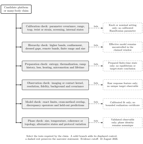
Validity map for analog model realization. Calibration, forward prediction, held-out agreement, and physical phase inference are separate evidential levels. A failure preserves the strongest narrower statement rather than forcing a binary platform verdict. Original schematic, not to scale; platform evidence is bounded through 10 August 2026.

Error budgets and adversarial controls

Separate at least four error classes:

Error class	Examples	Required test
Hamiltonian calibration	Lattice depth, scattering length, detuning, twist, range	Independent spectroscopy or response; covariance propagation
Model discrepancy	Higher bands, longer-range couplings, Floquet terms, bath coupling	Bound operators by scale and test an observable sensitive to each
State preparation	Entropy, defects, ramp excitations, inhomogeneity, history	Multiple thermometers, reverse or varied ramps, longer holds
Observation	Point spread, parity projection, loss, finite pulse, background	Calibrated response matrix and injected known states

Adversarial controls should be scientifically plausible. Deliberately increase a higher-band population, detune a resonance, shorten a thermalization hold, add a known imaging blur, or move into a regime where a benchmark method is exact. A validation procedure that continues to report success under such faults is not sensitive to the claimed failure mode.

Xu et al. 2025, main text, Methods, and source data illustrate both strength and ceiling. At half filling, long-range correlations were compared with controlled calculations after detailed trap and parameter calibration. At finite doping, comparison relied partly on approximate constrained-path calculations, so solver discrepancy joined experimental uncertainty. The platform can produce valuable predictions in that regime, but the evidence class must retain this distinction.

The evidence assessment is current through 10 August 2026. New benchmark windows, cross-platform comparisons, corrections, and contested phase inferences belong in the Quantum Matter and Emergence Research synthesis. The canonical cold-atom and synthetic-matter claim test matrix provides the chapter-wide semantic record. A reproducible verification workflow implements covariance propagation, ideal-versus-platform predictions, held-out tests, and a predeclared rejection path.

Exercise

A held-out falsification. A simulator predicts two observables $y_1(\theta)=\theta$ and $y_2(\theta)=2\theta+c$, where $c$ is an omitted discrepancy. Calibration on $y_1^{\mathrm{cal}}=1.00\pm0.02$ gives $\hat\theta=1.00$. A held-out measurement gives $y_2^{\mathrm h}=2.20\pm0.04$, while calibration uncertainty contributes $2\sigma_\theta=0.04$ to $y_2$. Ignoring other covariance, compute the standardized held-out residual under the target model $c=0$.

Solution

The target prediction is $2\hat\theta=2.00$. Experimental and propagated calibration variances add:

$$\sigma_{\mathrm h}= \sqrt{0.04^2+0.04^2} \simeq0.0566.$$

Thus

$$z=\frac{2.20-2.00}{0.0566}\simeq3.54, \qquad \chi_{\mathrm h}^2=z^2\simeq12.5.$$

The target-only model fails this predeclared held-out check at conventional thresholds. The result does not show that the apparatus is uncontrolled: fitting the discrepancy gives $c\simeq0.20$, after which a new independent observable is needed to validate the extended platform Hamiltonian.

References

• Elben, A., Vermersch, B., van Bijnen, R., Kokail, C., Brydges, T., Maier, C., Joshi, M. K., Blatt, R., Roos, C. F., and Zoller, P. (2020). “Cross-platform verification of intermediate scale quantum devices.” Physical Review Letters 124, 010504. doi:10.1103/PhysRevLett.124.010504.
• Hauke, P., Cucchietti, F. M., Tagliacozzo, L., Deutsch, I., and Lewenstein, M. (2012). “Can one trust quantum simulators?” Reports on Progress in Physics 75, 082401. doi:10.1088/0034-4885/75/8/082401.
• Trotzky, S., Chen, Y.-A., Flesch, A., McCulloch, I. P., Schollwöck, U., Eisert, J., and Bloch, I. (2012). “Probing the relaxation towards equilibrium in an isolated strongly correlated one-dimensional Bose gas.” Nature Physics 8, 325–330. doi:10.1038/nphys2232.
• Xu, M., Kendrick, L. H., Kale, A., Gang, Y., Feng, C., Zhang, S., Young, A. W., Lebrat, M., and Greiner, M. (2025). “A neutral-atom Hubbard quantum simulator in the cryogenic regime.” Nature 642, 909–915. doi:10.1038/s41586-025-09112-w.