Ultracold Platforms, Scales, and Traps

An ultracold-gas result is controlled only after laboratory settings have been translated into dimensionless many-body scales. Atom number, trap frequencies, field settings, ramp times, loss rates, and imaging resolution are inputs; density, temperature, interaction parameters, dimensionality, equilibration, and the observation kernel determine the physical claim. This page constructs that translation for continuum gases in harmonic or box confinement and states when a local-density interpretation is valid.

Required background. Galilean fields and scales fixes nonrelativistic normalization and density scales. Thermal density operators and the KMS condition supplies the equilibrium-state criterion. Chemical potentials and finite-density ensembles supplies the grand-canonical and fixed-number descriptions.

The platform scale hierarchy

For particles of mass $m$ in an external potential $V_{\mathrm{tr}}(\mathbf r)$, a minimal continuum Hamiltonian is

$$H=\int \mathrm d^d r\, \psi^\dagger\!\left(-\frac{\hbar^2\nabla^2}{2m} +V_{\mathrm{tr}}(\mathbf r)-\mu\right)\psi+H_{\mathrm{int}}.$$

For a two-component three-dimensional Fermi gas with central density $n_0$, define

$$k_F=(3\pi^2n_0)^{1/3}, \qquad E_F=\frac{\hbar^2k_F^2}{2m}, \qquad T_F=\frac{E_F}{k_B}.$$

The convention is explicit: $n_0$ is the total density of both spin components. The same laboratory sample can have quite different dimensionless parameters at its center and edge. A useful minimum set is

Physical issue	Dimensionless control	Controlled limit
Degeneracy	$T/T_F$ or entropy per particle $S/(Nk_B)$	Both are reported; neither is inferred from cloud size alone
Contact interaction	$1/(k_Fa)$ and $k_Fr_e$	Range corrections small when $\lvert k_Fr_e\rvert\ll1$
Harmonic confinement	$\hbar\omega_i/E_F$	Many occupied trap levels and slow spatial variation
Dimensional reduction	$E_F/(\hbar\omega_\perp)$, $k_BT/(\hbar\omega_\perp)$	Both small for a frozen transverse mode
Finite size	$k_FL_i$ or $L_i/\xi$	Large compared with microscopic and correlation lengths
Loss and heating	$\Gamma_{\mathrm{loss}}\hbar/E_F$, $\dot E\,t_{\mathrm{obs}}/(NE_F)$	Small over preparation and observation
Dynamics	$t_{\mathrm{ramp}}E_F/\hbar$, $t_{\mathrm{hold}}E_F/\hbar$	Compared with relevant gaps and relaxation times, not merely $\hbar/E_F$
Imaging	$k_F\Delta x$, $\Delta t\,E_F/\hbar$, detection fidelity	Forward model resolves the claimed wavelength and time scale

The table is a starting point rather than a universal checklist. In a lattice, $t$, $U$, the band gap, and superexchange replace some continuum scales; for molecules, internal-state and two-body loss scales enter; near criticality, the correlation length and critical slowing-down time dominate. Bloch, Dalibard, and Zwerger 2008, §§II–IV review the continuum and lattice scales, while Hadzibabic and Dalibard 2011, §§2–4 make the two-dimensional confinement and phase-space conditions explicit.

The chapter structure figure makes the logical order visible. Inspect the middle step: calibration determines an effective Hamiltonian with uncertainties, but preparation and observation must still be validated before the Hamiltonian can be used to identify a state.

On a narrow screen, swipe or use the Left and Right arrow keys to pan across the figure. Home and End move to its edges. A full-size link is also available.

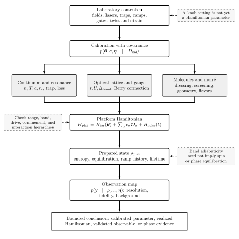
Platform-to-model dictionary. Laboratory knobs become physical parameters only through calibration, and the resulting Hamiltonian becomes an experimental claim only after state-preparation and observable maps pass scale-separation tests. Original schematic, not to scale; evidence status is bounded through 10 August 2026.

Text description of this diagram · Figure data (JSON)

Traps and the local-density map

For a harmonic trap,

$$V_{\mathrm{tr}}(\mathbf r)=\frac{m}{2} \sum_{i=1}^{d}\omega_i^2x_i^2, \qquad \mu(\mathbf r)=\mu_0-V_{\mathrm{tr}}(\mathbf r).$$

The local-density approximation (LDA) replaces a small region by a homogeneous equilibrium system at $\mu(\mathbf r)$ and $T$. If the homogeneous equation of state is $n_{\mathrm{hom}}(\mu,T,\lambda)$ for interaction parameters $\lambda$, then

$$n(\mathbf r)=n_{\mathrm{hom}}\!\left(\mu_0-V_{\mathrm{tr}}(\mathbf r),T,\lambda\right), \qquad N=\int \mathrm d^d r\,n(\mathbf r).$$

This is also an inverse calibration: a measured profile and a trusted homogeneous equation of state can determine $\mu_0$, $T$, and trap parameters. The approximation requires the potential to vary little over the longest relevant correlation length $\xi$,

$$\epsilon_{\mathrm{LDA}}(\mathbf r) =\frac{\xi(\mathbf r)\lvert\nabla\mu(\mathbf r)\rvert} {E_{\mathrm{loc}}(\mathbf r)}\ll1,$$

where $E_{\mathrm{loc}}$ is the energy scale controlling the local response. LDA can fail near a sharp digital-micromirror wall, close to a critical point where $\xi$ grows, in a small Mott domain, or when transport during preparation is too slow to establish local equilibrium. Homogeneous box traps, demonstrated for Fermi gases by Mukherjee et al. 2017, main text, reduce but do not eliminate boundary, preparation, and imaging corrections.

A trap-averaged signal is a different observable from the central homogeneous response. If the imaging kernel is $K(\mathbf R,\mathbf r)$ and the local response is $\mathcal O_{\mathrm{hom}}[\mu(\mathbf r),T]$, the measured quantity has the form

$$\mathcal O_{\mathrm{meas}}(\mathbf R) =\int \mathrm d^d r\, K(\mathbf R,\mathbf r)\, \mathcal O_{\mathrm{hom}}[\mu(\mathbf r),T] +b(\mathbf R).$$

The point-spread function, line-of-sight integration, parity projection, detection loss, and background $b$ belong in this forward model. Deconvolution without regularization and covariance propagation can create structure below the optical resolution.

Preparation, thermometry, and observation time

Thermometry is model-dependent in the deeply degenerate regime. Valid routes include fitting a dilute wing to a known equation of state, using fluctuation–dissipation relations with calibrated resolution, comparing short-range correlations to controlled calculations, or measuring an independently calibrated impurity or spin response. Agreement between at least two thermometers is stronger than a single best fit because trap, interaction, and imaging uncertainties are correlated.

Preparation has its own hierarchy. A ramp that is slow compared with a band gap may still be fast compared with spin exchange $J_{\mathrm ex}=4t^2/U$ or a critical relaxation time. Conversely, a fast quench can prepare a reproducible nonequilibrium state even though equilibrium language is then inappropriate. Record the full sequence, hold time, atom-number drift, energy deposition, and whether observed stationarity survives a longer hold.

The 2025 cryogenic Hubbard-gas experiment of Xu et al. 2025, main text and Methods illustrates this complete chain: trap shaping, lattice and field calibration, a low-entropy preparation, model-based thermometry, exact and approximate numerical comparisons, and explicit limits at finite doping were all needed to interpret the measured correlations. That result does not make every optical-lattice setting a low-temperature Hubbard realization.

Validity and interpretation

A scale table supports a calibrated platform description. It supports local equilibrium only where LDA, thermometry, and preparation checks pass. It supports a phase or transport statement only after the relevant observable kernel, finite-size and finite-time limits, loss, heating, and competing state preparations have been tested. Platform capabilities and benchmark status here are assessed through 10 August 2026. Mutable results and corrections are maintained in the Quantum Matter and Emergence Research synthesis.

The canonical cold-atom and synthetic-matter claim test matrix keeps each calibration, hierarchy, preparation, observable, and limit on the conclusion adjacent. A reproducible verification workflow should cover propagating calibration covariance through a model observable.

Exercise

Thomas–Fermi radius and LDA resolution. Consider a zero-temperature ideal two-component Fermi gas in an isotropic three-dimensional trap of frequency $\omega$. Its local Fermi energy is $E_F(\mathbf r)=\mu_0-\tfrac12m\omega^2r^2$ where positive. Find the cloud radius and the density profile. Which length should an imaging resolution $\Delta x$ be compared with near the edge?

Solution

The edge is defined by $E_F(R)=0$, hence

$$R=\sqrt{\frac{2\mu_0}{m\omega^2}}.$$

Using $n=k_F^3/(3\pi^2)$ and $\hbar^2k_F^2/(2m)=E_F$ gives

$$n(r)=\frac{1}{3\pi^2} \left[\frac{2m}{\hbar^2} \left(\mu_0-\frac12m\omega^2r^2\right)\right]^{3/2}$$

for $r<R$, and zero outside. Comparing $\Delta x$ only with the central $k_F^{-1}$ is insufficient near the edge. There the local Fermi wavelength grows, whereas the density-variation length shrinks: from $n\propto(R-r)^{3/2}$ one finds $L_n=n/\lvert\partial_r n\rvert\simeq 2(R-r)/3$. The forward model must resolve the smaller of the spatial feature being claimed and the local variation scale in the fitted region; LDA itself fails in the boundary layer where $k_F L_n$ is no longer large.

Nonvisual description of the synthetic-matter structure figure

This table states the relationships and qualifications shown in the figure above.

Figure element or arrow	Relation encoded	Condition or resulting statement
Laboratory controls	Fields, lasers, traps, ramps, gates, twist, and strain form the control vector $\mathbf u$.	The dashed side note states that a knob setting is not yet a Hamiltonian parameter.
Controls → calibration	Independent calibration produces a joint distribution $p(\boldsymbol\theta,\mathbf c,\boldsymbol\eta\mid D_{\rm cal})$.	Parameter, discrepancy, and nuisance covariances remain attached to later predictions.
Calibration → continuum and resonance branch	The continuum branch determines $n$, $T$, $a$, $r_e$, trap, and loss parameters.	Resonant universality requires the range, confinement, gradient, and lifetime hierarchy appropriate to the claim.
Calibration → optical-lattice and gauge branch	The lattice branch determines $t$, $U$, $\Delta_{\rm band}$, and the Berry connection.	Higher bands, nonadiabatic dressing, scalar potentials, and heating remain possible corrections.
Calibration → molecular and moiré branch	The molecular and moiré branch determines dressing, screening, geometry, and active flavors.	Internal channels, relaxation, remote bands, strain, and inhomogeneity constrain the reduction.
Three platform branches → platform Hamiltonian	Each branch feeds $H_{\rm plat}=H_{\rm tar}(\boldsymbol\theta)+\sum_\alpha c_\alpha\mathcal O_\alpha+H_{\rm noise}(t)$.	The dashed hierarchy condition requires checks of interaction range, band isolation, drive, confinement, and correction scales.
Platform Hamiltonian → prepared state	Hamiltonian realization is followed by preparation of $\rho_{\rm plat}$ with stated entropy, equilibration, ramp history, and lifetime.	The dashed side note warns that band adiabaticity need not imply spin or phase equilibration.
Prepared state → observation map	The state is mapped to $p(\mathbf y\mid\rho_{\rm plat},\boldsymbol\eta)$ with resolution, fidelity, and background.	Measurement inversion and covariance are distinct from Hamiltonian calibration.
Observation map → bounded conclusion	The completed chain supports only the strongest verified level: a calibrated parameter, realized Hamiltonian, validated observable, or phase evidence.	No later level follows solely from success at an earlier level.

References

• Bloch, I., Dalibard, J., and Zwerger, W. (2008). “Many-body physics with ultracold gases.” Reviews of Modern Physics 80, 885–964. doi:10.1103/RevModPhys.80.885.
• Hadzibabic, Z., and Dalibard, J. (2011). “Two-dimensional Bose fluids: An atomic physics perspective.” Rivista del Nuovo Cimento 34, 389–434. doi:10.1393/ncr/i2011-10066-3.
• Mukherjee, B., Yan, Z., Patel, P. B., Hadzibabic, Z., Yefsah, T., Struck, J., and Zwierlein, M. W. (2017). “Homogeneous atomic Fermi gases.” Physical Review Letters 118, 123401. doi:10.1103/PhysRevLett.118.123401.
• Xu, M., Kendrick, L. H., Kale, A., Gang, Y., Feng, C., Zhang, S., Young, A. W., Lebrat, M., and Greiner, M. (2025). “A neutral-atom Hubbard quantum simulator in the cryogenic regime.” Nature 642, 909–915. doi:10.1038/s41586-025-09112-w.