Feshbach Control and Resonance Calibration

A Feshbach-control setting is not itself a scattering length. The conversion requires a resonance parameterization, a calibrated local field, collision energy and confinement, and a loss and sweep protocol. The result is a many-body interaction window only after the range scale and density have also been specified.

Required background. Contact interactions and scattering length defines the low-energy amplitude and effective-range expansion. Nonrelativistic power counting and universality identifies the density and range parameters that control the contact limit. Tree-level matching and classical elimination supplies the logic for eliminating a detuned closed channel.

Field-to-scattering calibration

For an isolated magnetic resonance, a common signed convention is

$$a(B)=a_{\mathrm{bg}} \left(1-\frac{\Delta B}{B-B_0}\right).$$

Here $B_0$ is the pole position, $\Delta B$ is a signed width, $a_{\mathrm{bg}}$ is the background scattering length, and the zero crossing is $B_0+\Delta B$. Some experimental tables quote an unsigned width and encode the sign elsewhere; importing such a value without its convention can reverse which side is attractive. Chin et al. 2010, §§II–III review the two-channel origin, parameter conventions, and broad-versus-narrow classification.

Near the pole, field uncertainty is amplified:

$$\frac{\partial a}{\partial B} =a_{\mathrm{bg}}\frac{\Delta B}{(B-B_0)^2}, \qquad \sigma_a^2\simeq \left(\frac{\partial a}{\partial B}\right)^2\sigma_B^2 +\nabla_{\boldsymbol\theta}a^{\mathsf T} \Sigma_{\boldsymbol\theta} \nabla_{\boldsymbol\theta}a,$$

where $\boldsymbol\theta=(a_{\mathrm{bg}},B_0,\Delta B)$ and $\Sigma_{\boldsymbol\theta}$ includes their covariance. Spatial field curvature makes $a$ position dependent; temporal noise makes it stochastic. The relevant calibration is therefore the field distribution sampled by the atoms, not only a magnet power-supply reading.

The two-body amplitude at relative momentum $k$ is

$$f(k)=\frac{1}{-a^{-1}+\tfrac12r_e k^2-ik+O(k^4R^3)}.$$

At density scale $k_F$, the contact description requires $\lvert k_Fr_e\rvert\ll1$ and $k_FR\ll1$ in addition to the desired value of $1/(k_Fa)$. For a two-channel resonance, a useful positive range scale is

$$R^*=\frac{\hbar^2} {m\lvert a_{\mathrm{bg}}\delta\mu\,\Delta B\rvert},$$

where $\delta\mu$ is the open–closed-channel magnetic-moment difference. A broad resonance has $k_FR^*\ll1$ over the sample; a narrow resonance retains appreciable energy dependence and closed-channel physics. At the pole one often has $r_e\simeq-2R^*$ only within the isolated-resonance, low-energy approximation.

The structure diagram locates this calibration before the many-body Hamiltonian. Inspect the range branch: setting $a^{-1}=0$ removes one relevant inverse length but does not set $r_e$, confinement, or loss to zero.

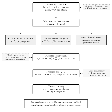
Resonance calibration within the platform-to-model chain. A pole in $a(B)$, the unitary many-body regime, and an acceptably long-lived preparation are separate statements. Original schematic, not to scale; experimental status is bounded through 10 August 2026.

Many-body unitarity, confinement, and losses

For a homogeneous three-dimensional gas, “unitarity” at finite density means

$$\lvert k_Fa\rvert^{-1}\ll1, \qquad \lvert k_Fr_e\rvert\ll1, \qquad k_FR\ll1,$$

over the occupied momentum and spatial distributions. The pole field $B_0$ need not coincide with the field that minimizes an observable correction in a trapped, finite-temperature, or narrow-resonance sample. Thermal momentum $k_T=\sqrt{mk_BT}/\hbar$ can replace $k_F$ in a dilute wing, so one must bound both $k_Fr_e$ and $k_Tr_e$ where relevant.

Tight confinement changes the scattering problem. In a harmonic transverse potential with oscillator length $a_\perp=\sqrt{\hbar/(m\omega_\perp)}$, virtual transverse excitations renormalize the effective low-dimensional coupling and can generate a confinement-induced resonance Olshanii 1998, pp. 938–941. Using the free-space $a(B)$ directly in a one-dimensional or quasi-two-dimensional Hamiltonian misses this matching step.

Loss supplies an independent clock. For a three-body loss coefficient $K_3$ in a locally homogeneous gas,

$$\dot n=-K_3n^3, \qquad \Gamma_3=K_3n^2.$$

A coherent many-body process of scale $E_*$ requires $\hbar\Gamma_3/E_*\ll1$ over the actual density history, not merely at the final central density. Two-body molecular loss, photon scattering for optical resonances, and heating during a field ramp enter analogously. Loss can also bias the surviving ensemble toward lower density, so a postselected equation of state is not automatically the closed-system one.

Association sweeps and calibration evidence

Sweeping through the pole can associate atom pairs into weakly bound dimers, but conversion is protocol dependent; Köhler, Góral, and Julienne 2006, §§V–VI review the two-body and many-body sweep regimes. In a two-level Landau–Zener reduction, the diabatic probability has the form

$$P_{\mathrm{diab}}=\exp\!\left[ -\frac{2\pi\lvert g\rvert^2} {\hbar\lvert\delta\mu\,\dot B\rvert} \right].$$

This expression identifies the adiabaticity parameter; a many-body gas adds pair correlations, density inhomogeneity, Pauli blocking, loss, and nonisolated levels. Molecule fraction therefore cannot be inverted into a unique temperature or closed-channel fraction without a forward model.

Precision coupled-channel spectroscopy can fix $B_0$, $\Delta B$, and bound-state energies jointly. Zürn et al. 2013, main text and supplemental analysis demonstrated such a calibration for lithium by combining molecular binding energies and scattering information. Current platform-specific parameters, overlapping-resonance fits, and optical-resonance loss budgets remain mutable. The evidence considered here is current through 10 August 2026; updated determinations belong in the Quantum Matter and Emergence Research synthesis.

The canonical cold-atom and synthetic-matter claim test matrix records field covariance, range, confinement, loss, preparation, and the maximum justified claim. A reproducible workflow should carry the few-body matching and its calibration uncertainties through to the platform observable.

Exercise

Uncertainty near a resonance. Take $a_{\mathrm{bg}}=-100a_0$, $\Delta B=-10\,\mathrm G$, $B-B_0=0.50\,\mathrm G$, and an uncorrelated field uncertainty $\sigma_B=5\,\mathrm{mG}$. Find $a$ and the field-induced standard uncertainty $\sigma_a$. Does quoting the pole position alone determine whether the gas is universal?

Solution

The signed formula gives

$$a=-100a_0\left(1-\frac{-10}{0.50}\right) =-2100a_0.$$

The derivative magnitude is

$$\left|\frac{\partial a}{\partial B}\right| =\left|\frac{(-100a_0)(-10\,\mathrm G)} {(0.50\,\mathrm G)^2}\right| =4000\,\frac{a_0}{\mathrm G},$$

so $\sigma_a=20a_0$ from field noise alone. Parameter covariance, field gradients, and calibration bias would add further uncertainty. The pole position does not determine universality: one must also evaluate $1/(k_Fa)$, $k_Fr_e$ or $k_FR^*$, thermal and trap distributions, confinement, and loss.

References

• Chin, C., Grimm, R., Julienne, P., and Tiesinga, E. (2010). “Feshbach resonances in ultracold gases.” Reviews of Modern Physics 82, 1225–1286. doi:10.1103/RevModPhys.82.1225.
• Köhler, T., Góral, K., and Julienne, P. S. (2006). “Production of cold molecules via magnetically tunable Feshbach resonances.” Reviews of Modern Physics 78, 1311–1361. doi:10.1103/RevModPhys.78.1311.
• Olshanii, M. (1998). “Atomic scattering in the presence of an external confinement and a gas of impenetrable bosons.” Physical Review Letters 81, 938–941. doi:10.1103/PhysRevLett.81.938.
• Zürn, G., Lompe, T., Wenz, A. N., Jochim, S., Julienne, P. S., and Hutson, J. M. (2013). “Precise characterization of $^6$Li Feshbach resonances using trap-sideband-resolved RF spectroscopy of weakly bound molecules.” Physical Review Letters 110, 135301. doi:10.1103/PhysRevLett.110.135301.