Integrable Charges and Generalized-Ensemble Model Tests

A generalized Gibbs ensemble (GGE) represents an integrable steady macrostate only when its conserved charges distinguish all root-density degrees of freedom relevant to the initial state. Commutativity and conservation are necessary but not sufficient: a truncated or ultralocal charge family can leave different string or rapidity distributions indistinguishable.

Required background. Root densities, macrostates, and observables supplies the charge-to-root-density map. Generalized Gibbs ensembles and integrable charges supplies the maximum-entropy construction.

Helpful background. Prethermalization and generalized ensembles distinguishes an exact integrable stationary ensemble from a long-lived approximate one.

From conserved charges to a macrostate

Let mutually commuting extensive charges satisfy

$$[Q_i,Q_j]=0, \qquad [H,Q_i]=0.$$

The generalized ensemble is

$$\rho_{\mathrm{GGE}} =\frac1Z\exp\!\left(-\sum_i\beta_iQ_i\right), \qquad Z=\operatorname{Tr} \exp\!\left(-\sum_i\beta_iQ_i\right).$$

For Bethe quasiparticle species $a$ with bare charge eigenvalues $h_{i,a}(\lambda)$, the charge densities are

$$\mathsf q_i= \sum_a\int\mathrm d\lambda\, \rho_{\mathrm p,a}(\lambda)h_{i,a}(\lambda).$$

The generalized driving term is

$$w_a(\lambda)=\sum_i\beta_i h_{i,a}(\lambda).$$

In a fermionic-style TBA convention compatible with the chapter’s positive scattering kernel, the saddle equations have the form

$$\epsilon_a(\lambda) =w_a(\lambda) -\sum_b\int\frac{\mathrm d\mu}{2\pi} K_{ab}(\lambda,\mu) \ln\!\left[1+e^{-\epsilon_b(\mu)}\right], \qquad n_a=\frac{1}{1+e^{\epsilon_a}}.$$

Statistics signs, parity factors, and string multiplicities are model data. Matching only the displayed algebra while importing a kernel from another convention can reconstruct the wrong filling.

The mathematical requirement for completeness is injectivity of the map

$$\{\rho_{\mathrm p,a}(\lambda)\} \longmapsto \{\mathsf q_i\}$$

within the allowed symmetry, energy-density, and regularity class. Numerically, one tests the singular spectrum of the discretized charge matrix and predicts held-out charges or observables. A small residual for the fitted charges is weak evidence if the inverse problem has a large null space.

Local, quasilocal, and symmetry-resolved charges

In the Lieb–Liniger gas, polynomial one-particle eigenvalues $h_j(k)=k^j$ formally encode moments of the rapidity distribution. Moment convergence and uniqueness still require tail conditions; finite data never determine an arbitrary distribution exactly. In lattice spin chains, the traditional transfer-matrix charges can be incomplete because different string species share the same ultralocal data. Essler and Fagotti 2016, §§3–5 review how this issue enters quench stationary states.

Ilievski et al. 2015, main text and supplemental charge construction showed that quasilocal charges are required for a complete GGE description of the spin-$1/2$ Heisenberg chain. Their result corrects a particular incomplete ensemble; it does not imply that one universal list works for every integrable model, boundary condition, or symmetry sector.

Initial-state symmetries restrict the admissible macrostate. Odd charges may vanish by parity, spin-reversal sectors may decouple, and degeneracies can preserve coherences not represented by a diagonal root-density ensemble. If proposed constraints do not commute, $\exp(-\sum_i\beta_iQ_i)$ remains a possible maximum-entropy state, but simultaneous sharp-charge reasoning and standard scalar TBA need not apply; stationarity also requires the full exponent to commute with $H$.

The structure figure makes the charge-completeness gate explicit. Inspect the branch from root densities to the ensemble: it must be reversible on the state class used, not merely capable of reproducing energy and particle number.

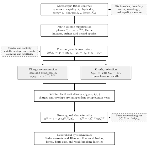
Charge-completeness and GGE dictionary. Conservation, linear independence, convergence, species coverage, and initial-state symmetry are separate requirements. Original schematic, not to scale.

Model tests for a GGE claim

A concrete test should:

1. Declare every quasiparticle species and rapidity measure.
2. Compute initial charge densities with finite-size and boundary corrections.
3. Reconstruct the root densities with regularization fixed independently of the desired observable.
4. Check positivity of $\rho_{\mathrm p}$ and $\rho_{\mathrm h}$, entropy, energy, particle number, and symmetry.
5. Predict charges and local observables not used in the fit.
6. Increase charge and species cutoffs and report the null space and covariance.
7. Compare with a quench-action or direct time-evolution result where available.

The original GGE proposal of Rigol et al. 2007, main text identifies conserved-mode constraints as the reason a generic thermal ensemble fails after an integrable quench. The strongest conclusion of a successful model test is that a specified charge-complete ensemble reproduces specified stationary local observables in a stated thermodynamic and long-time limit. It is not proof of microscopic equilibration or of an ordinary Gibbs temperature.

The canonical integrable-matter claim test matrix records species, charge completeness, entropy, initial input, and finite-size tests. A reproducible verification workflow tests charge-matrix rank, cutoff convergence, and held-out reconstruction.

Exercise

Why finitely many moments are incomplete. Consider two normalized symmetric rapidity measures:

$$\rho_A(k)=\frac12\delta(k-1)+\frac12\delta(k+1),$$

and

$$\rho_B(k)=\frac34\delta(k) +\frac18\delta(k-2)+\frac18\delta(k+2).$$

Compare their first four moments.

Solution

Both are normalized and symmetric, so

$$M_0=1,\qquad M_1=M_3=0.$$

Their second moments are also equal:

$$M_2[\rho_A]=1, \qquad M_2[\rho_B] =\frac18(2^2)+\frac18((-2)^2)=1.$$

But

$$M_4[\rho_A]=1, \qquad M_4[\rho_B] =\frac18(2^4)+\frac18((-2)^4)=4.$$

Thus particle number, momentum, and energy-like moments do not determine the macrostate. Delta measures idealize narrow packets; smoothing them preserves the lesson. A complete charge family must remove such null directions within the physically allowed class.

References

• Essler, F. H. L., and Fagotti, M. (2016). “Quench dynamics and relaxation in isolated integrable quantum spin chains.” Journal of Statistical Mechanics: Theory and Experiment 2016, 064002. doi:10.1088/1742-5468/2016/06/064002.
• Ilievski, E., De Nardis, J., Wouters, B., Caux, J.-S., Essler, F. H. L., and Prosen, T. (2015). “Complete generalized Gibbs ensembles in an interacting theory.” Physical Review Letters 115, 157201. doi:10.1103/PhysRevLett.115.157201.
• Rigol, M., Dunjko, V., Yurovsky, V., and Olshanii, M. (2007). “Relaxation in a completely integrable many-body quantum system: An ab initio study of the dynamics of the highly excited states.” Physical Review Letters 98, 050405. doi:10.1103/PhysRevLett.98.050405.