Quantum-Dot Transport and Impurity Spectroscopy

In linear response, a proportionately coupled Anderson quantum dot has a conductance determined by its equilibrium local spectral function, weighted by lead asymmetry and the thermal window. This exact interface does not extend automatically to finite bias, where the spectral function and distribution become nonequilibrium objects. A zero-bias ridge is compatible with Kondo screening but can also arise from resonant levels, superconducting Andreev processes, inelastic cotunnelling, or background channels.

Required background. The Anderson impurity model supplies the dot spectrum and lead widths. Strong-coupling phase shifts supplies the zero-temperature limit.

Helpful background. Kubo response supplies the equilibrium limit.

Linear conductance from equilibrium spectra

Let $\Gamma=\Gamma_L+\Gamma_R$ in the convention $G_d^R=(\omega-\varepsilon_d+i\Gamma)^{-1}$ for a noninteracting wide-band level. With proportional lead couplings and no interfering direct path,

$$\mathcal A_d(\omega)=-\frac{1}{\pi}\operatorname{Im}G_d^R(\omega)$$

is the unit-normalized local density of states. It is related to the chapter-2 convention by $A_d=2\pi\mathcal A_d$. The conductance is

$$G(T)=\frac{2e^2}{h} \frac{4\Gamma_L\Gamma_R}{\Gamma^2} \int\mathrm d\omega\, \left(-\frac{\partial f}{\partial\omega}\right) \pi\Gamma \mathcal A_d(\omega,T).$$

This normalization reproduces the resonant-level transmission. At $T=0$, the Friedel relation gives

$$G(0)=\frac{2e^2}{h} \frac{4\Gamma_L\Gamma_R}{\Gamma^2}\sin^2\delta.$$

Thus a screened symmetric dot reaches $2e^2/h$ only for symmetric lead coupling and negligible series or parallel resistance. The contact calibration must not be adjusted after seeing the desired value. Ng and Lee 1988, pp. 1768–1771 derives the low-temperature resonant Kondo transport limit.

The finite-bias current has the Meir–Wingreen structure. Under special proportional-coupling conditions it can be written using the interacting nonequilibrium spectral function, but $A_d(\omega,V)$ itself depends on bias. Substituting the equilibrium spectrum at large $eV$ is uncontrolled. Meir and Wingreen 1992 states the exact current interface and assumptions.

Coulomb blockade and Kondo regimes

When $T,\Gamma\ll U$, charge-degeneracy points form Coulomb-blockade peaks and fixed-charge valleys. In an odd-occupancy local-moment valley, lowering $T$ below $T_K$ can produce a zero-bias conductance ridge. A valid identification checks:

• odd–even valley structure and calibrated charging energies;
• universal temperature and magnetic-field crossover using a declared $T_K$ convention;
• approach to the Friedel phase-shift limit with measured lead asymmetry;
• splitting under Zeeman energy relative to temperature and width;
• absence or modelled presence of superconductivity, phonons, extra levels, and Fano paths; and
• reproducibility across gate trajectories without selecting only favorable cuts.

Bias spectroscopy maps voltage to dot excitation energy only after the voltage-drop lever arms and capacitance network are known. Peak height is convolved with temperature, lock-in excitation, lifetime, and instrument response.

Evidence ceiling

A conductance peak is an observable, not a quasiparticle name. The strongest equilibrium Kondo conclusion combines occupancy, scale collapse, phase-shift-compatible conductance, and a solver calculation for the calibrated Anderson model. Nonequilibrium splitting and satellites require a dedicated Keldysh or validated numerical treatment.

The validity diagram routes the impurity spectrum through contacts and measurement before interpretation.

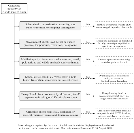
Linear-response conductance can be tied to an equilibrium spectral function under proportional coupling. Finite bias, background paths, and alternative zero-bias mechanisms require separate forward models. Original schematic, not to scale.

See the impurity claim test matrix for the spectroscopy stopping rule.

Exercise

Thermal-window check. At $T=0$, show that the conductance integral selects the Fermi-level spectrum.

Solution

As $T\to0$, $-\partial f/\partial\omega\to\delta(\omega)$. The integral becomes $\pi\Gamma \mathcal A_d(0)$. Under Fermi-liquid hypotheses, $\pi\Gamma \mathcal A_d(0)=\sin^2\delta$. This reduction fails if the lead couplings are not proportional, an interfering path contributes, or the measurement is outside linear response.

References

• Meir, Y., and Wingreen, N. S. (1992). “Landauer formula for the current through an interacting electron region.” Physical Review Letters 68, 2512–2515. doi:10.1103/PhysRevLett.68.2512.
• Ng, T.-K., and Lee, P. A. (1988). “On-site Coulomb repulsion and resonant tunneling.” Physical Review Letters 61, 1768–1771. doi:10.1103/PhysRevLett.61.1768.