Quenched Disorder and Disorder Averaging

Quenched disorder is sampled once and held fixed while the quantum or thermal degrees of freedom evolve. The correct observable is therefore computed at fixed disorder and averaged only afterward. This ordering distinguishes $\overline{\ln Z_V}$ from $\ln \overline{Z_V}$, fixes which correlation functions are normalized before averaging, and exposes when rare samples invalidate a statement based only on a typical realization.

Required background. Coherent-state path integrals supplies the Euclidean many-body functional integral. Thermal density operators and KMS supplies the fixed-Hamiltonian ensemble whose disorder average is taken.

Helpful background. Connected correlators and cumulants supplies the cumulant expansion used below.

Random fields and the order of averages

Let a static scalar potential $V(\mathbf x)$ couple to the density,

$$S_V=S_0+\int_0^\beta d\tau\int d^d x\,V(\mathbf x)n(\tau,\mathbf x).$$

An ensemble is part of the model. A common Gaussian choice has

$$\overline{V(\mathbf x)}=0, \qquad \overline{V(\mathbf x)V(\mathbf y)}=\Delta C(\mathbf x-\mathbf y),$$

where $C$ is positive as a covariance kernel. White noise means $C(\mathbf r)=\delta^{(d)}(\mathbf r)$ only below a declared ultraviolet cutoff; correlated disorder retains a finite correlation length $\zeta$. The distribution tail, not just $\Delta$, controls rare regions; Lifshits, Gredeskul, and Pastur 1988, ch. 1 develops this ensemble-to-spectrum distinction.

For each realization, $Z_V=\operatorname{Tr}e^{-\beta H[V]}$ and $\langle O\rangle_V=Z_V^{-1}\operatorname{Tr}(Oe^{-\beta H[V]})$. Quenched quantities are

$$F_{\mathrm q}=-T\,\overline{\ln Z_V}, \qquad \overline{\langle O\rangle_V},$$

not $-T\ln\overline{Z_V}$ and not a ratio of separately averaged numerator and denominator. Jensen’s inequality gives $F_{\mathrm q}\ge F_{\mathrm a}$ for the annealed free energy $F_{\mathrm a}=-T\ln\overline{Z_V}$. The distinction is physical: annealing lets the disorder equilibrate with the matter.

The chapter’s dependency structure is summarized in the following original diagram. Inspect the first arrow: the ensemble and order of averages precede every replica, sigma-model, localization, or glass conclusion.

On a narrow screen, swipe or use the Left and Right arrow keys to pan across the figure. Home and End move to its edges. A full-size link is also available.

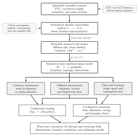
From quenched input to localization observables. Solid arrows add a derivation; dashed annotations mark ensemble, symmetry, dimension, or scale assumptions. The diagram is schematic and not a phase diagram.

Text description of this diagram · Figure data (JSON)

Cumulants and disorder-induced interactions

For a general distribution, introduce connected disorder cumulants $K_p$. Averaging a source $J$ gives

$$\ln \overline{e^{\int J V}} =\sum_{p=1}^\infty\frac{1}{p!} \int K_p(x_1,\ldots,x_p)J(x_1)\cdots J(x_p).$$

For the centered Gaussian ensemble only $K_2=\Delta C$ survives. Because the Euclidean coupling supplies $J(\tau,\mathbf x)=-n(\tau,\mathbf x)$, averaging the unnormalized Boltzmann factor produces

$$\overline{e^{-\int Vn}} =\exp\!\left[ \frac{\Delta}{2}\int d^d x\,d^d y\,C(\mathbf x-\mathbf y) \int_0^\beta d\tau\,d\tau'\,n(\tau,\mathbf x)n(\tau',\mathbf y) \right].$$

The two independent imaginary times express static disorder. In an effective action the same term appears with a minus sign because the weight is $e^{-S_{\mathrm{eff}}}$. This sign and the double-time structure are useful checks on replica calculations.

Self-averaging and rare samples

For an extensive sample observable $X_L$, define

$$R_X(L)=\frac{\overline{X_L^2}-(\overline{X_L})^2}{(\overline{X_L})^2}.$$

$R_X\to0$ is self-averaging in the chosen ensemble and limit. It can fail at a random critical point or for observables dominated by broad tails; averages, medians, typical values $X_{\mathrm{typ}}=\exp\overline{\ln X}$, and full distributions then answer different questions. Aharony and Harris 1996 show why critical randomness can prevent strong self-averaging.

Rare-region estimates must retain the tail that creates them. A region of volume $\ell^d$ may occur with probability $p(\ell)\sim e^{-c\ell^d}$ while its relaxation time grows as $\tau(\ell)\sim e^{b\ell^d}$; eliminating $\ell$ produces a power-law distribution of times. Replacing the ensemble by its variance alone can erase this physics.

The canonical disorder and glass claim test matrix records which ensemble, limit, and negative test accompany each later claim.

Exercise

Quenched versus annealed. Let $V$ be a centered Gaussian variable with variance $\Delta$ and let a toy realization have $Z_V=e^{aV}$. Compute $F_{\mathrm q}$ and $F_{\mathrm a}$.

Solution

Since $\ln Z_V=aV$, $\overline{\ln Z_V}=0$ and $F_{\mathrm q}=0$. The Gaussian moment-generating function gives $\overline{Z_V}=e^{a^2\Delta/2}$, so $F_{\mathrm a}=-Ta^2\Delta/2$. Thus $F_{\mathrm q}\ge F_{\mathrm a}$, with strict inequality for $a^2\Delta>0$.

Nonvisual description of the disorder structure figure

This table states the relationships and qualifications shown in the figure above.

Figure element or arrow	Relation encoded	Condition or resulting statement
Quenched ensemble	The construction begins with $P[V]$, its correlation length and symmetries, and the order of thermodynamic and disorder limits.	The dashed side condition distinguishes $\overline{\ln Z}$ from $\ln\overline Z$; self-averaging alone does not justify equality.
Ensemble → normalized observables	Disorder observables are normalized by replicas with $n\to0$ or by boson–fermion supersymmetry.	The representation is fixed before any diffusive or localization approximation.
Normalization side condition	Convergence, analytic continuation, and rare-sample tails constrain the normalization step.	Failure preserves only the directly defined disorder average, not a controlled replica or supersymmetric continuation.
Normalized observables → retarded–advanced soft modes	Weak static disorder produces diffusons and, when symmetry permits, cooperons with pole $(Dq^2-i\omega)^{-1}$.	This arrow assumes the weak-disorder regime.
Soft modes → nonlinear sigma model	The long-wavelength modes are organized into a symmetry-class field $Q$ with $Q^2=1$ and gradient, frequency, topological, and interaction terms.	The displayed expansion requires $q\ell\ll1$ and $\lvert\omega\rvert\tau\ll1$.
Sigma model → interference branch	Cooperon structure produces weak localization or antilocalization.	The sign and channel count depend on symmetry, dephasing, magnetic field, and spin–orbit scales.
Sigma model → interaction branch	Diffusive density and spin modes produce Altshuler–Aronov corrections and Finkel’stein flow.	Interaction amplitudes and frequency renormalization must use the same normalization as the diffusive action.
Sigma model → class and topology branch	The target space and allowed topological term follow from the symmetry class.	The conclusion remains dimension-, boundary-, and energy-specific.
Interference and interaction branches → conductance scaling	Their controlled corrections feed $\beta(g)=\mathrm d\ln g/\mathrm d\ln L$.	A perturbative logarithm is not itself a critical point.
Interaction plus class/topology branches → localization statement	These branches determine which class-, dimension-, energy-, and boundary-fixed localization statement is admissible.	Conductance scaling and localization statements jointly require finite-size fits of relevant and irrelevant drift, distributions, boundary conditions, and dephasing cutoffs.

References

• Amnon Aharony and A. Brooks Harris, “Absence of Self-Averaging and Universal Fluctuations in Random Systems near Critical Points,” Physical Review Letters 77 (1996) 3700–3703. DOI
• Ilya M. Lifshits, Sergei A. Gredeskul, and Leonid A. Pastur, Introduction to the Theory of Disordered Systems, Wiley, 1988. WorldCat