

NRG and CT-QMC Impurity Solvers: Validity and Error
Numerical renormalization group (NRG) and continuous-time quantum Monte Carlo (CT-QMC) answer complementary questions about an impurity model. NRG follows the flow across exponentially separated energy scales and supplies real-frequency transitions, but it approximates the bath, truncates states, and usually broadens a discrete spectrum. CT-QMC samples a continuous-time diagrammatic expansion without Trotter error, but it returns noisy imaginary-time or Matsubara data and may suffer from autocorrelation and a sign problem. Analytic continuation adds a separate inverse-problem uncertainty. A credible comparison therefore freezes one action and one observable, exposes each solver’s controls, and meets first on quantities that require neither NRG broadening nor Monte Carlo continuation.
Required background. The Anderson model supplies a shared benchmark. Convergence certification and covariance and resampling supply numerical error discipline.
Helpful background. Spectral moments supplies exact high-frequency checks.
Freeze the benchmark before choosing a solver
Section titled “Freeze the benchmark before choosing a solver”Use the spin-degenerate Anderson model and specify the bath through the same hybridization function in both codes. A concrete interacting benchmark is
with a flat, particle–hole-symmetric bath of half-bandwidth , zero field, and energies measured from the chemical potential. The bath-edge convention and the definition of are part of the input, not implementation details.
This benchmark has exact checks before either solver runs:
- particle–hole and spin symmetry give and ;
- fermionic anticommutation gives ;
- the leading high-frequency terms are
- at , each solver must reproduce the exact resonant-level result for the bath representation it actually uses,
where is that representation’s hybridization function. CT-QMC checks the specified continuous-bath target directly. For NRG, each calculation first checks the corresponding discretized ; only the controlled and -averaged limit is compared with the continuous-bath result.
The interacting comparison below uses the local susceptibility
at zero field. This is not the thermodynamic impurity susceptibility . Comparing one definition from NRG with the other from CT-QMC would create a solver discrepancy before any numerics begin.
How NRG reaches exponentially small scales
Section titled “How NRG reaches exponentially small scales”For a discretization parameter and shift , NRG groups the positive and negative bath energies into intervals whose edges scale as . A unitary transformation maps one representative mode from each interval to a Wilson chain with asymptotic hopping
so adding site resolves a characteristic scale
The Hamiltonian is diagonalized iteratively. After each site is added, high rescaled-energy multiplets are discarded so the next Hilbert space remains finite. Those discarded states are not simply thrown away when observables are evaluated. Each discarded shell state is tensored with the untouched states of the later Wilson-chain “environment”; the union over shells forms the complete approximate many-body basis. The full-density-matrix construction then assigns the appropriate thermal and environment weight to each shell. Anders and Schiller 2005, pp. 196801-1–196801-4 supplies the complete-basis construction; Weichselbaum and von Delft 2007, Eqs. (5)–(13) develops the full density matrix.
An NRG convergence grid changes one control at a time:
- vary and increase the number of interleaved shifts;
- depending on the implementation, increase the number of kept multiplets, raise the rescaled energy cutoff, or tighten a separately defined discarded-weight tolerance;
- exploit exact symmetries without accidentally removing perturbations under study;
- move the temperature relative to the shell scale and verify known fixed-point spectra; and
- compare exact sum rules and moments before applying a spectral kernel.
The discarded-weight diagnostic estimates whether important density-matrix support lies near the truncation boundary; it is a convergence indicator, not a rigorous error bound. Weichselbaum 2011, §§II–III defines this diagnostic.
For a fermionic operator , complete-basis transitions give discrete Lehmann weights. Evaluate directly from those unbroadened poles,
Here denotes the appropriate full-density-matrix probability, including its shell and environment weight. Broadening is a later visualization or reconstruction step. A log-Gaussian width, its crossover to a linear kernel near , and averaging can change a peak height or width without changing the underlying poles. Integrated weights and high-frequency moments should converge before pointwise line shapes are trusted. Bulla, Costi, and Pruschke 2008, §§II–IV reviews the discretization, truncation, thermodynamics, and spectral constructions.
What CT-HYB and CT-INT actually sample
Section titled “What CT-HYB and CT-INT actually sample”CT-HYB expands the partition function in the impurity–bath hybridization. A configuration contains an ordered set of impurity creation and annihilation times; its weight is a local many-body trace times a determinant of hybridization functions connecting those times. CT-INT instead expands in interaction vertices, and its configuration weight contains a determinant of noninteracting propagators. The two algorithms are continuous in imaginary time, so there is no time-slice extrapolation, but their expansion orders, matrix conditioning, sign behavior, and efficient parameter regimes differ. Werner et al. 2006, Eqs. (2)–(5) introduces CT-HYB; Rubtsov, Savkin, and Lichtenstein 2005, §§II–III develops CT-INT.
Successive Monte Carlo configurations are correlated. For a scalar estimator , define
Blocking lengths must exceed the measured autocorrelation scale, and independent replicas should agree. A vector such as needs its full covariance matrix: nearby time bins are not independent data points.
If weights have signs or phases, sampling gives
The variance grows rapidly as the average sign decreases; more samples do not change that exponential complexity. The report therefore includes warmup, update acceptance and ergodicity tests, expansion-order distribution, matrix-stabilization checks, , binning, independent replicas, covariance, and average sign or phase. Gull et al. 2011, §§II, V, and IX compares the algorithm families and their error mechanisms.
Imaginary-axis information and continuation
Section titled “Imaginary-axis information and continuation”A measured imaginary-time Green function is related to the local spectrum by
Here is the unit-normalized local density of states used throughout this impurity chapter; equivalently, the volume-wide spectral convention is . The kernel exponentially suppresses fine real-frequency structure, so many distinct spectra fit noisy within its covariance. No increase in sample count turns analytic continuation into a well-conditioned inversion.
A continuation result inherits its default model or prior, regularizer, frequency grid, covariance treatment, and hyperparameter choice. Validate it by (i) forward transforming the proposed spectrum into or , including covariance; (ii) predicting held-out imaginary-axis points; (iii) testing synthetic spectra with comparable noise and resolution; and (iv) checking moments not imposed as priors. Normalizing during continuation is not an independent validation of that normalization. Jarrell and Gubernatis 1996, §§2–4 explains the inverse problem and maximum-entropy regularization.
The next figure separates raw solver outputs from reconstruction-dependent spectra.
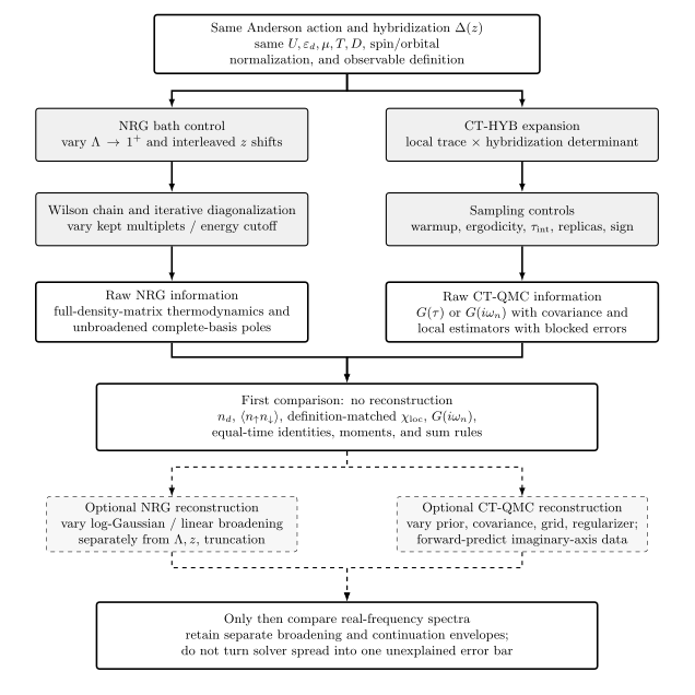
Cross-solver validation begins before either real-frequency reconstruction. NRG supplies unbroadened complete-basis poles and CT-QMC supplies imaginary-axis estimates with their covariance; they first meet at definition-matched thermodynamics, , and exact moments. Broadened NRG and analytically continued CT-QMC spectra are compared only after their separate reconstruction controls pass. Original workflow schematic; not to scale.
The same relationships in a text-first form are:
| Stage | NRG lane | CT-HYB lane | Comparison or error rule |
|---|---|---|---|
| Frozen input | represent the declared by intervals and a Wilson chain | expand the same continuous-bath action in hybridization events | hold , spin/orbital normalization, and observable definitions fixed |
| Numerical controls | vary , interleaved shifts, chain length, kept multiplets or energy cutoff, and symmetries | test warmup, acceptance, ergodicity, matrix stabilization, , binning, replicas, covariance, and average sign | keep discretization/truncation envelopes distinct from blocked sampling errors and sign diagnostics |
| Raw output | full-density-matrix thermodynamics and unbroadened complete-basis poles | or with covariance and local estimators with blocked errors | retain the native representation and its correlations |
| First merge | direct pole sums or transforms | direct imaginary-axis and equal-time estimators | compare , double occupancy, definition-matched , , identities, moments, and sum rules with no broadening or continuation |
| Optional real-frequency reconstruction | vary log-Gaussian/linear kernels separately from , and truncation | vary prior or default model, covariance treatment, grid, regularizer, and hyperparameter | forward-test each reconstruction, then retain separate broadening and continuation envelopes |
| Real-frequency comparison | broadened NRG | continued CT-HYB | compare only after the separate controls pass; never collapse both reconstruction envelopes into one unexplained error bar |
A definition-matched cross-solver benchmark
Section titled “A definition-matched cross-solver benchmark”For the frozen particle–hole-symmetric benchmark, compare quantities that require no continuation or broadening first:
For the unit-normalized local spectrum, define . Then per spin, and particle–hole symmetry makes for this benchmark.
| Observable | NRG check | CT-QMC check | Shared convention |
|---|---|---|---|
| Occupancy | full-density-matrix trace, stable under , and truncation | direct/equal-time estimator with covariance | spin sum; exact value here |
| Double occupancy | unbroadened operator expectation | local estimator with blocked error | same , and action sign |
| the same imaginary-time local-spin correlator or its Lehmann integral | integrated local-spin correlator with covariance | field couples only to ; not | |
| direct transform of unbroadened complete-basis poles | direct Matsubara estimator | same Fourier sign and frequency grid | |
| Spectral weight and first moment | pole sums and large- coefficients | equal-time discontinuity and large- fit | per spin and here |
For an NRG observable , report separate envelopes from , truncation, and—where relevant—thermal-shell placement. For a CT-QMC scalar, report the blocked statistical error, replica spread, sign, and any estimator or tail-fit variation. For use the CT-QMC covariance rather than treating frequencies as independent. If a combined uncertainty is quoted, state whether independent components were added in quadrature or conservative envelopes were added linearly; a truncation envelope is not automatically a Gaussian standard deviation.
A useful discrepancy diagnostic for a scalar is
means the declared conservative intervals overlap; it does not certify that both methods are unbiased. For a Matsubara vector, inspect the residual with the CT-QMC covariance and repeat the NRG control grid. Only after , double occupancy, , , and the moments agree should one compare a real-frequency Kondo width. That last comparison must retain an NRG broadening envelope and a CT-QMC continuation ensemble separately.
The chapter structure diagram places both solvers after the model and its candidate fixed-point classification but before observable inference: numerical flow must test the candidate branch rather than assume it.
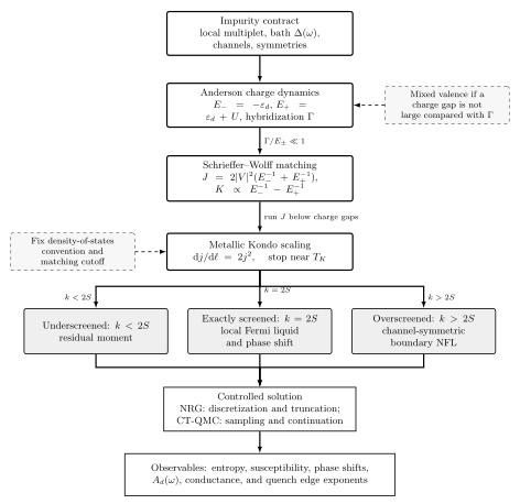
NRG or CT-QMC must verify the candidate infrared branch and quantify solver-specific errors before observable inference. The one-orbital Anderson route supplies one active hybridization eigenchannel; multichannel branches require separate microscopic input. Original workflow schematic, not to scale.
The impurity claim test matrix states the solver-specific stopping rules.
Common pitfalls
Section titled “Common pitfalls”Lowering an NRG energy cutoff to “keep more.” In the common rescaled-energy convention, increasing the cutoff keeps more states. Only a separately defined discarded-weight tolerance is reduced.
Comparing different susceptibilities. and answer different questions and can differ substantially.
Transforming a broadened NRG plot to Matsubara frequency. Use the unbroadened complete-basis poles. Broadening is not part of the Hamiltonian and should not contaminate a continuation-free comparison.
Using a continuation constraint as its own check. A unit-normalized spectrum proves nothing about if unit normalization was imposed. Check the equal-time discontinuity or the leading Matsubara coefficient independently.
Exercises
Section titled “Exercises”Estimate the required Wilson-chain length. With and , approximately which iteration reaches ?
Solution
Solve . Since ,
This is only a scale estimate. The usable resolution also depends on averaging, truncation, temperature, and the observable.
Convert autocorrelation into effective samples. A CT-HYB run records measurements with . Estimate . If the average sign is , what rough sign-reweighted scale warns about the variance?
Solution
The autocorrelation estimate is
Sign reweighting often inflates variance roughly as . The corresponding warning scale is . This is not a universal error formula, but it shows why the raw measurement count is misleading.
Check the symmetric high-frequency moment. Show why the coefficient of vanishes for at spin symmetry.
Solution
Spin and particle–hole symmetry give . Hence
Both solvers must therefore approach . A nonzero fitted first moment points to insufficient high-frequency range, a bath/action mismatch, broken symmetry, or an estimator error.
Diagnose a false agreement. NRG and CT-QMC give the same occupancy, but their real-frequency peak widths disagree by 30%. List the next variations.
Solution
For NRG, vary , averaging, kept-state threshold, and broadening kernel separately, checking moments after each change. For CT-QMC, inspect covariance and autocorrelation, vary statistics, continuation method, default model, frequency grid, and synthetic-recovery tests. Compare directly before continuing. Occupancy agreement validates one integral but cannot determine a narrow spectral width.
References
Section titled “References”- Anders, F. B., and Schiller, A. (2005). “Real-time dynamics in quantum-impurity systems: A time-dependent numerical renormalization-group approach.” Physical Review Letters 95, 196801. doi:10.1103/PhysRevLett.95.196801.
- Bulla, R., Costi, T. A., and Pruschke, T. (2008). “Numerical renormalization group method for quantum impurity systems.” Reviews of Modern Physics 80, 395–450. doi:10.1103/RevModPhys.80.395.
- Gull, E., Millis, A. J., Lichtenstein, A. I., Rubtsov, A. N., Troyer, M., and Werner, P. (2011). “Continuous-time Monte Carlo methods for quantum impurity models.” Reviews of Modern Physics 83, 349–404. doi:10.1103/RevModPhys.83.349.
- Jarrell, M., and Gubernatis, J. E. (1996). “Bayesian inference and the analytic continuation of imaginary-time quantum Monte Carlo data.” Physics Reports 269, 133–195. doi:10.1016/0370-1573(95)00074-7.
- Rubtsov, A. N., Savkin, V. V., and Lichtenstein, A. I. (2005). “Continuous-time quantum Monte Carlo method for fermions.” Physical Review B 72, 035122. doi:10.1103/PhysRevB.72.035122.
- Weichselbaum, A. (2011). “Discarded weight and entanglement spectra in the numerical renormalization group.” Physical Review B 84, 125130. doi:10.1103/PhysRevB.84.125130.
- Weichselbaum, A., and von Delft, J. (2007). “Sum-rule conserving spectral functions from the numerical renormalization group.” Physical Review Letters 99, 076402. doi:10.1103/PhysRevLett.99.076402.
- Werner, P., Comanac, A., de’ Medici, L., Troyer, M., and Millis, A. J. (2006). “Continuous-time solver for quantum impurity models.” Physical Review Letters 97, 076405. doi:10.1103/PhysRevLett.97.076405.