Chemical Potentials and Finite-Density Ensembles

A chemical potential weights charge sectors through $H-\mu Q$. For a free relativistic gas it replaces the particle and antiparticle Boltzmann exponents by $E_{\mathbf p}\mp q\mu$, changes KMS detailed balance, and generates density and susceptibility by derivatives of the grand potential. Fermions remain normalizable for any finite $\mu$ at fixed regulator, while an uncondensed bosonic ensemble fails when $\lvert q\mu\rvert$ reaches the lightest charged energy.

The chemical-potential shifts and finite-density thermal conventions used below are derived in Laine and Vuorinen 2016, §§ 3.3–3.5.

Required background. Conserved Charges and Grand-Canonical States states the stability conditions. Thermal Propagators and Spectral Representations supplies thermal weights. Helpful background. Partition Functions and Thermodynamic Response supplies derivative identities.

Free relativistic distributions

For charge $q>0$, define

$$n_B^\pm(\mathbf p)= \frac1{e^{\beta(E_{\mathbf p}\mp q\mu)}-1}, \qquad n_F^\pm(\mathbf p)= \frac1{e^{\beta(E_{\mathbf p}\mp q\mu)}+1},$$

where $+$ labels particles of charge $+q$ and $-$ antiparticles of charge $-q$. The net charge densities are

$$n_Q^{B,F}=q\int\frac{\mathrm d^{d-1}p}{(2\pi)^{d-1}} \left(n_{B,F}^+-n_{B,F}^-\right)$$

after the vacuum charge is consistently subtracted. The corresponding grand-potential densities are

$$\begin{aligned} \frac{\Omega_B}{V} &=T\int_{\mathbf p} \left[ \log(1-e^{-\beta(E_{\mathbf p}-q\mu)}) +\log(1-e^{-\beta(E_{\mathbf p}+q\mu)}) \right],\\ \frac{\Omega_F}{V} &=-gT\int_{\mathbf p} \left[ \log(1+e^{-\beta(E_{\mathbf p}-q\mu)}) +\log(1+e^{-\beta(E_{\mathbf p}+q\mu)}) \right], \end{aligned}$$

where $\int_{\mathbf p}=\int\mathrm d^{d-1}p/(2\pi)^{d-1}$ and $g$ counts declared internal degrees of freedom. Differentiation checks $n_Q=-V^{-1}\partial_\mu\Omega$.

Susceptibility and stability

The isothermal charge susceptibility is

$$\chi_Q=\frac{\partial n_Q}{\partial\mu} =\beta q^2\int_{\mathbf p} \left[ n^+(1\pm n^+)+n^-(1\pm n^-) \right],$$

with the upper sign for bosons and lower sign for fermions. It is nonnegative in the stable free ensemble. An interacting susceptibility matrix must include operator mixing and contact terms, and a negative eigenvalue of the homogeneous thermodynamic Hessian signals that the assumed branch is unstable or constrained incorrectly.

For bosons, $E_{\mathbf0}-q\mu\to0$ makes $n_B^+$ diverge. In infinite volume the excess charge enters a condensate and the equation of state must be rewritten with the order parameter. For fermions at $T=0$, occupation approaches a step function $\theta(q\mu-E_{\mathbf p})$, producing a Fermi surface when $q\mu>m$.

KMS with physical and modular time

Let $A$ lower the charge by $q_A$, so

$$[Q,A]=-q_AA.$$

If $A(t)$ evolves with the physical Hamiltonian $H$, grand-canonical KMS becomes

$$G_A^>(\omega)= e^{\beta(\omega-\mu q_A)}G_A^<(\omega).$$

If evolution is instead generated by $K=H-\mu Q$, the factor is $e^{\beta\omega_K}$. The two frequency variables satisfy $\omega_K=\omega_H-\mu q_A$. Stating the generator prevents the same physical excitation from being assigned two apparently inconsistent thresholds.

Chemical-potential convention and domain table

The table compares equivalent finite-density descriptions only after their time generator, charge convention, and domain of validity are declared; its last column gives the quantity that must agree when translating between them.

Representation	Declared object	Domain check	Invariant comparison
Grand-canonical trace	$e^{-\beta(H-\mu Q)}$	$K$ bounded sufficiently for normalization	charge density $-V^{-1}\partial_\mu\Omega$
Physical-$H$ KMS	factor $e^{\beta(\omega-\mu q_A)}$ for $[Q,A]=-q_AA$	charge and adjoint fixed	detailed balance after translating frequency
Modular-$K$ KMS	factor $e^{\beta\omega_K}$	same state, $K$-time declared	$\omega_K=\omega_H-\mu q_A$
Euclidean derivative	$\partial_\tau-q\mu$ in the convention used here	contour and field charge fixed	same Matsubara denominator as the trace
Thermal twist	$\widetilde\Phi(\beta)=e^{-\beta q\mu}\widetilde\Phi(0)$ after removing $D_\tau=\partial_\tau-q\mu$	nonunitary for real $\mu$	returns the same shifted spectrum
Imaginary chemical potential	$\mu=i\theta T$	charge lattice and large-gauge period	Wilson holonomy $e^{iq\theta}$, inverse field gluing $e^{-iq\theta}$
Fixed density	Legendre transform from $\Omega(\mu)$	convexity and phase coexistence	matching $n=-V^{-1}\partial_\mu\Omega$

This table is the canonical semantic reference for the chapter. Holonomy and method pages link back rather than silently choosing a different $i$ or charge sign.

Common pitfalls

Chemical potential called an energy shift without a charge convention. Only $\mu q$ is invariant under rescaling $Q\to cQ$, $\mu\to\mu/c$.

Vacuum subtraction applied to density onset. Removing a temperature-independent zero-point energy is not permission to remove the physical threshold or filled Fermi sea.

Bosonic divergence ignored. Continuing the normal-phase distribution beyond $q\mu=m$ produces an ill-defined ensemble, not a high-density perturbative result.

The schematic below organizes the relationships used on this page. Inspect it with this question in mind: Which charge structures license chemical potentials or generalized equilibrium states?

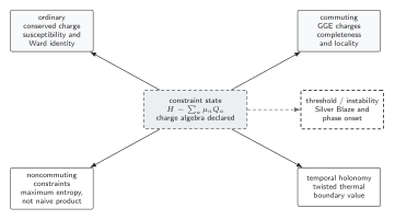
A grand-canonical state requires conserved charges and a declared algebra; commuting integrable charges, noncommuting constraints, temporal holonomies, and density thresholds demand distinct constructions and checks. Connections classify the charge structure and required construction; their direction is organizational, not a causal-time ordering. Dashed marks show qualifications and failure boundaries. The diagram is schematic and not to scale.

The surrounding discussion supplies the relevant equations and checks in text form; the figure is a navigational summary.

Exercise

At $T=0$ in three spatial dimensions, show that a free Dirac gas with degeneracy $g$ has number density $n=g p_F^3/(6\pi^2)$, $p_F=\sqrt{\mu^2-m^2}$ for $\mu>m$.

Solution

The Fermi distribution becomes $\theta(\mu-E_{\mathbf p})$, so occupied momenta form a ball of radius $p_F$. Thus $n=g\int_{\lvert\mathbf p\rvert<p_F}\mathrm d^3p/(2\pi)^3=g(4\pi p_F^3/3)/(2\pi)^3=g p_F^3/(6\pi^2)$. Below $\mu=m$ the ball is empty.

References

• Kapusta, Joseph I., and Charles Gale. Finite-Temperature Field Theory: Principles and Applications. 2nd ed. Cambridge: Cambridge University Press, 2006. doi:10.1017/CBO9780511535130.
• Laine, Mikko, and Aleksi Vuorinen. Basics of Thermal Field Theory. Cham: Springer, 2016. doi:10.1007/978-3-319-31933-9; Open PDF.
• Le Bellac, Michel. Thermal Field Theory. Cambridge: Cambridge University Press, 1996. doi:10.1017/CBO9780511721700.