Convergence, Extrapolation, and Error Certification

A truncation result is certified only to the level supported by independent tests: a rigorous variational bound, a justified asymptotic extrapolation, or empirical stability over declared regulator variations. Certification requires more than a smooth plot. It combines fixed-axis cutoff sequences, correlated fits, residuals or variances, counterterm and fit-model enlargement, held-out observables, and agreement between genuinely different bases. Any untested axis remains a systematic limitation rather than a zero error.

Required background. Renormalizing a Truncated Hamiltonian supplies the matching and counterterm protocol. Variational Principles and Field-Theory Ansätze supplies bounds, residuals, and ansatz error. Observables and Dynamics in Truncated Spaces supplies effective-operator, spectral-sum, leakage, and time-window errors.

Helpful background. Complete Lattice Error Budgets supplies error-source decomposition. Correlated Fits, Model Selection, and Stability Tests supplies covariance-aware inference and fit-stability methods.

A convergence claim begins with identifiable axes

Convergence and certification contract. Freeze the target observable and matching inputs; list every independent Hilbert, volume, basis-scale, counterterm, variational, state, operator, time, and numerical cutoff; derive or justify the asymptotic model; retain correlations; predeclare fit windows and alternatives; reserve held-out observables; and state whether the final evidence is a bound, an asymptotic extrapolation, empirical stability, or an unresolved finite-cutoff result.

Let $\boldsymbol\epsilon$ collect small regulator variables such as $E_{\max}^{-1}$, $N^{-1}$, $e^{-mL}$, a basis incompleteness parameter, an operator-basis remainder, and a time-step. A local asymptotic model may have the form

$$O(\boldsymbol\epsilon) =O_*+\sum_i a_i\epsilon_i^{p_i} +\sum_{i<j}a_{ij}\epsilon_i^{p_i}\epsilon_j^{p_j} +\cdots.$$

The exponents must come from perturbation theory, an OPE or effective-tail analysis, a theorem, or comparison among prespecified alternatives. Choosing the exponent that produces the desired intercept is not uncertainty quantification.

A dimensionless diagonal sequence such as $E_{\max}/m=2N=4mL$ cannot identify the three coefficients or their cross terms. At least one fixed-axis scan for each consequential regulator is needed. When a full Cartesian grid is unaffordable, the unestimated interaction between axes belongs explicitly in the error statement.

Correlated fits preserve shared information

Cutoff points often share bare inputs, perturbative coefficients, calibration data, stochastic samples, or a common higher-cutoff reference. Their uncertainties are correlated. For a linearized model $\mathbf y=X\boldsymbol \beta+\boldsymbol\eta$ with covariance $C$, generalized least squares gives

$$\widehat{\boldsymbol\beta} =(X^{T}C^{-1}X)^{-1}X^{T}C^{-1}\mathbf y, \qquad \operatorname{Cov}(\widehat{\boldsymbol\beta}) =(X^{T}C^{-1}X)^{-1}.$$

Dropping off-diagonal entries can either inflate or shrink the intercept uncertainty and changes the goodness-of-fit test. If $C$ is estimated and ill-conditioned, record the resampling, shrinkage, or singular-value prescription and vary it as part of the analysis.

Fit-model uncertainty is assessed by prespecified changes: remove the lowest cutoff, add the next asymptotic term, vary a theoretically allowed exponent, and compare correlated residuals. Information criteria or model averaging can summarize these alternatives, but they do not rescue a family that omits the true leading term. The statistical foundations and limitations of model-selection uncertainty are treated by Claeskens and Hjort 2008, Chapters 2–4.

Exactly checkable two-basis extrapolation

Consider two synthetic basis sequences with a common exact limit,

$$M_A(\Lambda)=1+\frac{2}{\Lambda^2}+\frac{3}{\Lambda^3}, \qquad M_B(\Lambda)=1-\frac{1}{\Lambda^2}+\frac{4}{\Lambda^4}.$$

They approach the same mass gap from opposite sides:

Analytic mass-gap sequences used to test an extrapolation pipeline.

Λ	MA	MB
8	1.037109375	0.985351563
10	1.023000000	0.990400000
12	1.015625000	0.993248457
16	1.008544922	0.996154785
20	1.005375000	0.997525000

A correct joint model gives the shared intercept $M_*=1$ while allowing basis-specific coefficients and subleading powers. For the simpler exact form $M(\Lambda)=M_*+a\Lambda^{-p}$, two cutoffs related by $s>1$ give the Richardson estimator

$$M_*= \frac{s^pM(s\Lambda)-M(\Lambda)}{s^p-1}.$$

Applying this with $p=2$ to the displayed sequences leaves the declared $\Lambda^{-3}$ or $\Lambda^{-4}$ remainder, which can be predicted exactly. This benchmark checks data ingestion, cutoff powers, shared-intercept design, and uncertainty code without relying on any physical simulation.

The physically relevant next step is a finite-volume interacting mass gap in two bases—for example, free-energy and conformal bases—with the same renormalization inputs. Agreement before translating volume, operator normalization, and matching schemes is not cross-basis evidence.

Residuals answer only the question they measure

For a computed eigenpair $(\widetilde E,|\widetilde\psi\rangle)$ in a fixed finite matrix,

$$r_{\mathrm{eig}} =\frac{\|H_\Lambda\widetilde\psi-\widetilde E\widetilde\psi\|} {\|H_\Lambda\|\,\|\widetilde\psi\|}$$

tests the numerical eigensolver. It says nothing about $H_\Lambda-H_{\mathrm{target}}$. A variational energy variance probes the state residual in the Hamiltonian being measured, but it too can omit directions outside a prior field regulator or use an approximate $H^2$.

Useful residuals form a hierarchy:

• algebraic residuals: Hermiticity, constraints, selection rules, eigenpairs;
• variational residuals: energy variance and tangent-orthogonal components;
• matching residuals: input conditions after refitting at each cutoff;
• asymptotic residuals: correlated deviations from the cutoff model;
• physical residuals: held-out sum rules, Ward identities, matrix elements, phase shifts, or cross-formulation observables.

No residual should be relabeled as another. In particular, an eigensolver tolerance of $10^{-12}$ cannot justify twelve digits in a continuum mass.

Certification has four evidence levels

Rigorous bound. State the theorem and hypotheses. Nested Rayleigh–Ritz spaces can bound ordered discrete energies, while Temple-type lower bounds need a certified spectral gap. Most matrix elements and dynamics have no such automatic bound.

Asymptotic extrapolation. State the derived expansion, fitted cutoff range, covariance, subleading alternatives, and remainder estimate. Hamiltonian truncation studies of two-dimensional $\phi^4$ show how explicit leading and next-to-leading corrections alter the cutoff behavior Rychkov and Vitale 2015, §§ 3–4 and Elias-Miró, Rychkov, and Vitale 2017, §§ 2–4.

Empirical stability. State the tested hyperrectangle of cutoffs, bases, counterterm bases, volumes, optimizers, observables, and time windows. The claim is restricted to that range and benchmark set.

Unresolved. A nonmonotone sequence, model-dependent intercept, untested operator correction, or single-basis result may still be scientifically useful. It must be labeled as a finite-cutoff estimate or open systematic, not promoted to a certified continuum value.

The shared map contains the adversarial branch

Read the dashed branch as a required falsification test: if a fitted energy is flat while an unused observable drifts, enlarge the state and operator bases and redo the match. Certification lies after this loop, not at the plateau.

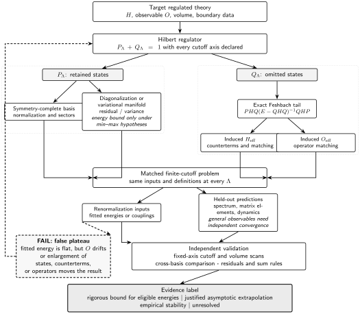
The convergence flow distinguishes monotone variational energy bounds from general observable convergence and routes a false fitted plateau back through state, counterterm, and effective-operator enlargement. Only independent cutoff axes, residuals, held-out predictions, and cross-basis agreement support the final evidence label. The diagram is schematic and not to scale.

Minimum truncation certification record

This is the central semantic form of the chapter-wide record. A result is reproducible only when every row has a concrete value or an explicit unresolved limitation.

Required fields for a truncation result and the test that can falsify each field.

Field	Required declaration	Independent test	Failure signal
Target	Hamiltonian, prior regulator, volume, boundary data, observable	Units and free or exact limit	Changing target across cutoff points
Projectors	PΛ, QΛ, all cutoff axes, limit order	State counts and nestedness	Unidentified omitted states
Basis and sectors	Normalization, Gram matrix, null removal, exact charges	Hermiticity and selection rules	Duplicates or broken constraints
Induced Hamiltonian	Derived operator basis and approximation order	Omitted-state toy model or perturbative coefficient	Drift incompatible with the declared tail
Counterterms	Inputs, running coefficients, and no-double-counting rule	Refit protocol at every cutoff	A fitted datum presented as a prediction
Variational status	Manifold, optimizer, symmetry, bound hypotheses	Residual, variance, and ansatz enlargement	Energy plateau with a large residual
Effective observables	Projected and induced operator terms	Sum rule or matched matrix element	Spectrum stable while the observable drifts
Cutoff sequence	Independent basis, volume, counterterm, time, and state scans	Fixed-axis and cross-term fits	Only one diagonal sequence
Extrapolation	Asymptotic form, fit window, covariance, alternatives	Window and model stability	Exponent chosen from the desired answer
Held-out tests	Unused spectrum, matrix element, dynamics, and second basis	Blind comparison after choices freeze	All tests participated in tuning
Adversarial enlargement	Larger state and operator bases	Repeat the full match and prediction	Former plateau moves beyond its error
Claim	Bound, asymptotic evidence, empirical stability, or unresolved	Error and cost reproduced independently	Precision exceeds the weakest test

Adversarial failure: a fitted false plateau

At each cutoff, tune a coefficient so that $E_0(\Lambda)=1$ exactly. The plot is perfectly flat by construction. Suppose the unused matrix element behaves as

$$O(\Lambda)=0.5+\frac{1}{\log\Lambda}.$$

Over a modest cutoff range it can also look nearly flat, yet its drift is parametrically slow and not represented by a polynomial in $1/\Lambda$. Adding a second effective operator may change both the drift and the fitted coefficient. A single polynomial fit with a tiny statistical error is then misleading.

The correct record says that the energy is a renormalization condition, not a prediction. The matrix element requires a tail analysis that permits logarithms, larger cutoffs, operator-basis enlargement, and a second Hilbert basis. If those tests disagree, the continuum intercept remains unresolved.

Observable-level validation checklist

• Freeze target, inputs, observable definitions, and analysis choices before revealing held-out reference values.
• Scan each consequential cutoff at fixed values of the others and include enough points to test at least one subleading term.
• Retain covariance from shared matching or reference data and test covariance regularization.
• Compare fit windows, theoretically allowed powers or logarithms, and correlated residuals; report model spread.
• Keep eigensolver, variational, matching, extrapolation, finite-volume, operator, and time-window errors separate.
• Repeat after enlarging the counterterm and effective-operator bases and after changing to a second complete Hilbert basis.
• Require held-out spectral and matrix-element or dynamical tests; internal cutoff stability alone is insufficient.
• Label the final result as a rigorous bound, asymptotic evidence, empirical stability, or unresolved, and quote no precision beyond the weakest test.

For the bounded LH5 calculation below, normal ordering is with respect to $H_0$ and the free-vacuum energy is set to zero. The reported first gap is $\Delta=E_{0,-}-E_{0,+}$, while the declared even-sector observable is

$$\overline O_2=\frac{1}{L}\int_0^L dx\,{:}\!\phi^2\!{:}, \qquad F_2=\left|\langle 0,+|\overline O_2|1,+\rangle\right|.$$

The minimal counterterm basis is $\{\mathbf 1,\int dx\,{:}\!\phi^2\!{:}\}$; vacuum and operator coefficients are varied separately. The $E_{\max}=24$ result is an internal, same-formulation regression frozen before lower-cutoff fits are inspected. It is not the later cross-method benchmark extension.

A useful finite-volume $1+1$-dimensional $\phi^4$ baseline sets $L=2\pi$, $m=1$, $g=0.5$ and $E_{\max}=8,10,12,14,16$, with exact $g=0$ checks and a separately frozen higher-cutoff interacting reference. Vacuum energy, first gap, $\phi^2$ matrix element, counterterm effects, cutoff residuals, and eigensolver residuals keep distinct tolerances. The higher-cutoff reference remains blind until the lower-cutoff method and fit choices are frozen.

You should now be able to (1) build a covariance-aware, multi-axis cutoff fit and test its asymptotic remainder against a two-basis analytic sequence, and (2) assign the strongest defensible evidence label using residual, counterterm, held-out-observable, and cross-basis tests. Benchmark Theories for Truncation Methods turns these criteria into a staged stress ladder. Statistical details remain in Statistical Inference and Error Budgets, rigorous spectral bounds continue in Mathematical QFT. Cross-formulation continuum tests continue in Hamiltonian Continuum Limits and Hamiltonian–Euclidean Cross-Validation, and dated performance comparisons belong to Research.

Exercises

Apply Richardson extrapolation

Suppose $M(\Lambda)=M_*+a/\Lambda^2$ exactly and the values at $\Lambda=10$ and $20$ are $1.02$ and $1.005$. Find $M_*$ and $a$.

Solution

Here $s=2$ and $p=2$, so

$$M_*=\frac{4M(20)-M(10)}3 =\frac{4(1.005)-1.02}{3}=1.$$

Then $a=10^2[M(10)-M_*]=2$. A third cutoff is still needed in practice to test whether an omitted subleading term invalidates the exact two-parameter model.

Identify the evidence class

A nested Ritz sequence gives ground energies $1.10,1.06,1.04$, a fitted extrapolation $1.01(2)$, and no effective-operator or cross-basis tests. Which statements are justified?

Solution

Under the min–max hypotheses, each finite-cutoff energy is a rigorous upper bound on the corresponding regulated target energy, and the monotone sequence is consistent with variational improvement. The number $1.01(2)$ is only an asymptotic extrapolation if its cutoff form, covariance, window, and remainder tests are justified; the three values alone do not establish that. No claim about matrix elements or general continuum certification is supported because effective-operator, independent-axis, and cross-basis tests are absent.

References

• Claeskens, Gerda, and Nils Lid Hjort. Model Selection and Model Averaging. Cambridge University Press, 2008. DOI.
• Elias Miró, Joan, Slava Rychkov, and Lorenzo G. Vitale. “NLO Renormalization in the Hamiltonian Truncation.” Physical Review D 96, 065024 (2017). DOI.
• Rychkov, Slava, and Lorenzo G. Vitale. “Hamiltonian Truncation Study of the $\phi^4$ Theory in Two Dimensions.” Physical Review D 91, 085011 (2015). DOI.