

Multistage Bayesian Global Inference and Evidence
A heavy-ion global analysis calibrates a computational model that maps fluctuating nuclear initial states through pre-equilibrium, viscous hydrodynamics, particlization, hadronic transport, and optionally rare probes to measured observables. Bayesian machinery makes the conditional uncertainty explicit; it cannot rescue an incomplete covariance, an invalid stage, a biased emulator, or a non-identifiable parameterization. The primary product is therefore a versioned posterior and its model/data provenance, not a best-fit curve.
Required background. Transport inverse problems and error budgets supplies identifiability and covariance, initial conditions supplies the first stage, and bulk evolution supplies the required downstream chain. Helpful background. Charge fluctuations, jets, electromagnetic probes, open heavy flavor, and quarkonium add typed optional probes.
Evidence status on this page was checked through 10 August 2026.
Conditional inference
Section titled “Conditional inference”Let denote model parameters, the complete model/version, and the selected measurements. Bayes’ theorem gives
For a Gaussian residual, a useful likelihood is
where and
The terms represent experimental covariance, finite-event simulation noise, emulator predictive covariance, and model discrepancy. They cannot generally be replaced by diagonal error bars. Correlated normalization systematics are often better represented by nuisance parameters than by adding independent variances.
The posterior is conditional on . A narrow posterior can result from an overly rigid parameterization or omitted discrepancy; precision is not automatically accuracy.
Design and emulation
Section titled “Design and emulation”Full event-by-event simulations are expensive, so an analysis evaluates a space-filling design , reduces correlated outputs if useful, and trains an emulator . A Gaussian-process or neural emulator must return predictive uncertainty, not only a mean.
Validation uses held-out full-model points. Standardized residuals,
should have the declared coverage and reveal no parameter-dependent structure. Good interpolation error averaged over outputs can hide a bias in the few combinations that control a transport coefficient, so validation should be performed in the likelihood metric.
The design must cover the posterior support. If sampling accumulates at a prior boundary or outside the convex region validated by full simulations, the remedy is additional design/model work, not trusting extrapolation.
Closure, posterior prediction, and identifiability
Section titled “Closure, posterior prediction, and identifiability”A closure test generates pseudodata at a hidden , passes it through the same covariance and emulator pipeline, and asks whether calibrated credible regions cover at the expected frequency. Closure on noiseless emulator output is too weak; the test should use independent full-model runs and realistic noise.
Posterior predictive checks draw
including nuisance and discrepancy terms. They test whether the fitted model reproduces held-out distributions and correlations, not merely means used in calibration.
Local identifiability is encoded by the sensitivity matrix . Small singular values of the whitened matrix
identify parameter combinations that data cannot distinguish. Reporting marginal intervals without the correlated directions can make a degeneracy look like several independent measurements.
Transfer across systems and beam energies
Section titled “Transfer across systems and beam energies”A joint calibration must distinguish parameters intended to be common properties of QCD matter from system-specific latent variables. A hierarchical model may share a transport function across collision systems while allowing nuclear geometry, longitudinal deposition, normalization, and detector nuisance parameters to vary. Simply multiplying likelihoods is valid only after cross-system experimental and theory correlations have been represented.
Beam-energy transfer is especially nontrivial. Lower energies introduce stronger baryon stopping, three-dimensional longitudinal structure, nonzero conserved-charge densities, diffusion, and a finite-density EOS; a boost-invariant zero-density stage graph cannot be carried over unchanged. A shared posterior is meaningful only on the intersection of the stages’ validity domains or after the energy-dependent extensions are parameterized and tested.
Small systems provide an even sharper boundary. Short lifetimes and gradients can enlarge nonhydrodynamic corrections, while initial-state correlations can mimic part of the final anisotropy. Including or data can improve discrimination, but it does not by itself prove that the same hydrodynamic truncation is valid there. The analysis must pass switching, constitutive-residual, and structural-alternative tests in each system before a common transport interpretation is claimed.
Heavy-ion global-inference provenance table
Section titled “Heavy-ion global-inference provenance table”This canonical table defines the minimum machine-readable record for bulk and typed probe analyses. A record fails schema validation when a required item is absent; “not evaluated” must be explicit.
| Record block | Required content | Reject or limit the claim when |
|---|---|---|
| Analysis identity | Immutable release, code/container versions, random seeds, checksums, evidence cutoff, supersession status | Results cannot be reproduced or the evidence date is unknown |
| Stage graph | Required bulk chain: ordered initial-state, pre-equilibrium, hydrodynamic, EOS, particlization, afterburner, detector-analysis versions and switch maps; optional probe branches explicitly marked | A stage or interface is unnamed, conservation is untested, or an optional probe is mistaken for a required bulk stage |
| Parameter schema | Names, units, transforms, domains, functional bases, shared/fixed parameters | A reported parameter changes meaning across stages or systems |
| Prior | Joint density including correlations, bounds, hyperpriors, and rationale | Posterior support is prior-boundary dominated without sensitivity analysis |
| Observable schema | Definition, units, cuts, centrality, species/feed-down, estimator, theory analysis code | Theory and experiment implement different observables |
| Dataset identity | Collaboration, collision system/energy, publication/data release, table/bin locator, revision | Points cannot be traced to a primary dataset |
| Experimental covariance | Statistical and correlated systematic covariance or nuisance construction, including cross-observable/system information | Diagonal approximation materially changes the posterior |
| Design and simulator noise | Design algorithm/points, event counts, convergence, , failed-run policy | Design misses posterior support or simulation noise is ignored |
| Emulator | Type, preprocessing, hyperparameters, predictive covariance, held-out points, coverage in likelihood metric | Bias or undercoverage is unresolved |
| Model discrepancy | Functional form/kernel, domain knowledge, hyperpriors, identifiability with physics parameters | Omitted discrepancy drives implausibly narrow or stage-dependent constraints |
| Closure | Blinded generator point/model, independent simulation, noise, coverage criterion and result | The pipeline cannot recover known parameters |
| Posterior products | Weighted samples, log likelihood/prior, nuisance draws, convergence diagnostics, evidence when claimed | Only a best fit or corner plot is released |
| Posterior prediction | Calibrated and held-out observables, full uncertainty, residual diagnostics | Key data are systematically missed |
| Alternative models | Initial states, , afterburners, kernels or model averaging, with common data/covariance | Claim is sensitive to one untested structural choice |
| Sensitivity and claim status | Whitened sensitivity/identifiable combinations; label as fit, constraint, preference, exclusion, or discovery | Language exceeds the tested discriminator |
| Typed probe discriminator | One of “bulk,” “jet,” “electromagnetic,” “open-heavy-flavor,” “quarkonium,” or a separately versioned extension | A probe record uses generic fields that erase its kernel |
| Jet extension | Hard /nuclear baseline, shower and medium kernels, recoil/response, reconstruction, covariance, validity domain, evidence cutoff | A transport claim lacks a factorized baseline, response model, or common observable definition |
| Electromagnetic extension | Current/emission-rate version, equilibrium/viscous domain, prompt/decay/pre-equilibrium baselines, acceptance, covariance, validity domain, evidence cutoff | Source attribution or temperature claim lacks a competing-source baseline |
| Open-heavy-flavor extension | Production/CNM baseline, Boltzmann/Langevin kernel and coefficients, radiative terms, fragmentation/coalescence, feed-down, covariance, validity domain, evidence cutoff | A diffusion claim lacks kernel definition or hadronization alternatives |
| Quarkonium extension | State/feed-down network, EFT hierarchy, open-system/rate kernel, formation, dissociation/regeneration, CNM baseline, covariance, validity domain, evidence cutoff | A potential/rate claim mixes incompatible hierarchies or omits regeneration |
The typed discriminator prevents physically different inverse problems from being represented as a generic “probe likelihood.” Each extension carries its own validity domain and the same evidence cutoff as the parent analysis.
What current analyses establish
Section titled “What current analyses establish”Multisystem JETSCAPE calibration showed that soft observables across RHIC and LHC can constrain parameterized shear and bulk viscosities while exposing sensitivity to particlization models Everett et al. 2021. An IP-Glasma-based analysis added a distinct initial-state family and explored transfer learning and model averaging Heffernan et al. 2024. A 2025 jet analysis extended Bayesian calibration to inclusive hadron and jet suppression Ehlers et al. 2025.
Recent methodology explicitly models theory discrepancy; controlled examples show that doing so can broaden or reconcile physics-parameter posteriors that otherwise appear inconsistent Jaiswal et al. 2025. This is not a license for an arbitrarily flexible discrepancy, which could absorb all parameter sensitivity. Its kernel and hyperpriors need physical justification and closure.
As of the cutoff, global analyses provide quantitative, reproducible, model-conditional constraints and comparisons. They do not deliver a unique reconstruction of the QGP’s microscopic dynamics, a model-independent viscosity curve, or Bayesian proof that one complete collision paradigm is true.
A minimal release workflow
Section titled “A minimal release workflow”- Freeze the stage graph, datasets, observable code, covariance, and priors.
- Run design simulations and numerical convergence checks.
- Validate emulator coverage on held-out full simulations.
- Pass blinded closure before looking at data posteriors.
- Sample with convergence diagnostics and retain weighted posterior products.
- Run posterior prediction, leave-one-system/observable-out tests, and prior/discrepancy sensitivity.
- Compare structural alternatives with the same dataset and covariance.
- Release the table record, data transformations, samples, and strongest supported claim.
The multistage graph is the forward map whose uncertainty model must accompany every global posterior.
On a narrow screen, swipe or use the Left and Right arrow keys to pan across the figure. Home and End move to its edges. A full-size link is also available.
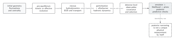
Each solid edge is a physical or statistical transformation that can add parameters, numerical error, and structural alternatives. The likelihood must compare detector-matched observables with the full experimental covariance and a validated emulator, while posterior predictive checks test withheld or replicated data. The dashed branch marks the key limitation: a narrow posterior is a conditional constraint unless alternative model structures are also resolved. The diagram is schematic and not to scale.
The text equivalent is to version every stage, validate the emulator and closure tests, retain correlated systematics and model discrepancy, state priors, test structural alternatives on the same data, and report the strongest conclusion that remains stable under those changes.
Global inference can combine probes only by retaining the six distinct physical branches shown here.
On a narrow screen, swipe or use the Left and Right arrow keys to pan across the figure. Home and End move to its edges. A full-size link is also available.
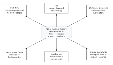
The common medium history creates useful cross-probe constraints and shared uncertainties, but each branch has a different operator, baseline, evolution kernel, acceptance, and model discrepancy. Quarkonium and charge cumulants are explicitly separate, as are quarkonium and open heavy flavor. A valid joint likelihood therefore preserves typed branch models and their block covariance rather than collapsing them into a generic probe term. The diagram is schematic and not to scale.
In text, share only physically common parameters and nuisance sources, retain branch-specific validity domains and evidence cutoffs, and test whether posterior constraints survive alternative kernels and medium histories. Apparent agreement across probes is not independent evidence if the same model error drives every branch.
Exercises
Section titled “Exercises”1. Correlated normalization. Two data points share a normalization uncertainty. Why is adding independently to each diagonal element wrong?
Solution
The uncertainty moves both points coherently, so it contributes an outer-product covariance , or an equivalent common nuisance parameter. A diagonal treatment permits opposite fluctuations and falsely increases shape uncertainty while decreasing correlation information.
2. Prior-bound posterior. A viscosity parameter’s posterior piles up at its lower prior bound. What can be concluded?
Solution
Only that, within the model and prior, likelihood support extends toward or beyond that boundary. One should expand a physically admissible prior, inspect model validity, emulator coverage, and degeneracies, and repeat sensitivity tests. Quoting the boundary as a measured value is unjustified.
Continue to the chapter overview to select the equilibrium, collision-stage, or probe-specific branch to which this inference record applies.
References
Section titled “References”- Ehlers, Raymond, et al. (JETSCAPE Collaboration). “Bayesian Inference Analysis of Jet Quenching Using Inclusive Jet and Hadron Suppression Measurements.” Physical Review C 111, no. 5 (2025): 054913. DOI.
- Everett, D., et al. (JETSCAPE Collaboration). “Multisystem Bayesian Constraints on the Transport Coefficients of QCD Matter.” Physical Review C 103, no. 5 (2021): 054904. DOI.
- Heffernan, Matthew, Charles Gale, Sangyong Jeon, and Jean-François Paquet. “Bayesian Quantification of Strongly Interacting Matter with Color Glass Condensate Initial Conditions.” Physical Review C 109, no. 6 (2024): 065207. DOI.
- Jaiswal, Sunil, Chun Shen, Richard J. Furnstahl, Ulrich Heinz, and Matthew T. Pratola. “Bayesian Model–Data Comparison Incorporating Theoretical Uncertainties.” Physics Letters B 870 (2025): 139946. DOI.
- Paquet, Jean-François. “Applications of Emulation and Bayesian Methods in Heavy-Ion Physics.” Journal of Physics G: Nuclear and Particle Physics 51, no. 10 (2024): 103001. DOI.