Partition Functions and Thermodynamic Response

A source-dependent partition function is a generating function for equilibrium thermodynamics. Its first derivatives give expectation values, its second derivatives give connected fluctuations and static response, and Legendre transforms exchange controlled sources for mean extensive variables. Every derivative must declare what is held fixed and how the source enters the exponent; otherwise even a correct formula can acquire the wrong sign or normalization.

The response identities and their equilibrium hypotheses descend from Kubo 1957, §§ 2–3, pp. 572–579.

Required background. Statistical Ensembles and Field Configurations defines the normalized measures used here. Helpful background. Current Sources and Generating Functionals gives the QFT source and Ward-identity framework.

One generating function, several thermodynamic potentials

For volume $V$, inverse temperature $\beta$, chemical potentials $\mu_a$, and a source $h$ coupled to an extensive observable $M$, define

$$\Xi(\beta,\mu_a,h) =\operatorname{Tr}\exp\!\left[-\beta \left(H-\sum_a\mu_aQ_a-hM\right)\right].$$

The Massieu function $\Psi=\log\Xi$ is dimensionless and the grand potential is

$$\Omega=-T\log\Xi=-pV$$

for a homogeneous system without additional boundary work. Differentiation at fixed $\beta,V$, and all other sources gives

$$\langle Q_a\rangle =\frac1\beta\frac{\partial\Psi}{\partial\mu_a}, \qquad \langle M\rangle =\frac1\beta\frac{\partial\Psi}{\partial h}, \qquad \langle H-\mu_aQ_a-hM\rangle =-\frac{\partial\Psi}{\partial\beta}.$$

The last derivative is not $\langle H\rangle$ when $\beta$ varies while $\mu_a$ and $h$ are held fixed. Equivalently one may use dimensionless sources $\alpha_a=\beta\mu_a$; translating between the two parameterizations changes which derivative is taken.

For a canonical partition function $Z(\beta,V)$,

$$F=-T\log Z, \qquad S=-\left(\frac{\partial F}{\partial T}\right)_V, \qquad E=F+TS, \qquad p=-\left(\frac{\partial F}{\partial V}\right)_T.$$

These relations assume that the regulator and boundary work are held consistently while differentiating. A lattice calculation that changes the lattice spacing with temperature needs an explicit line of constant physics; differentiating bare parameters as though they were fixed physical couplings does not yield the thermodynamic energy.

Connected cumulants and susceptibility matrices

Because $\Psi$ is the logarithm of the partition function, its source derivatives are connected cumulants:

$$\frac{\partial^2\Psi}{\partial h^2} =\beta^2\left(\langle M^2\rangle-\langle M\rangle^2\right).$$

For charge densities $n_a=\langle Q_a\rangle/V$, define the isothermal susceptibility matrix

$$\chi_{ab} =\left(\frac{\partial n_a}{\partial\mu_b}\right)_{T,V,\mu_{c\ne b}} =\frac{\beta}{V}\langle\delta Q_a\,\delta Q_b\rangle.$$

For Hermitian mutually commuting charges in a positive Gibbs state, $\chi$ is positive semidefinite. A negative eigenvalue therefore signals either an unstable homogeneous branch, a mismatched constraint, or an ineligible operator—not merely an unusual convention. With noncommuting charges, the relevant quantum response is an imaginary-time-ordered Kubo–Mori correlation rather than the naive equal-time covariance.

The heat capacity at fixed volume is another variance,

$$C_V=\left(\frac{\partial E}{\partial T}\right)_V =\frac{\langle(\Delta H)^2\rangle}{T^2},$$

provided $H$ has no explicit temperature dependence. Effective Hamiltonians with temperature-dependent matched coefficients require derivative terms from those coefficients.

Legendre transforms and convexity

The source $h$ and mean $m=\langle M\rangle/V$ are conjugate. In a differentiable finite-volume system one may define

$$g(h)=-\frac{T}{V}\log\Xi(h), \qquad f(m)=g(h)+hm, \qquad m=-\frac{\partial g}{\partial h}.$$

Then $\partial f/\partial m=h$ and

$$\frac{\partial m}{\partial h} =-\left(\frac{\partial^2 g}{\partial h^2}\right) =\frac{\beta}{V}\langle(\Delta M)^2\rangle\ge0.$$

At phase coexistence the infinite-volume function may not be differentiable. The correct transform is Legendre–Fenchel, and the inverse map can become set-valued. A metastable nonconvex effective potential can remain useful as a coarse-grained approximation, but it is not the exact convex thermodynamic Legendre transform.

Free scalar consistency check

For independent bosonic modes of frequencies $\omega_{\mathbf k}$,

$$\log Z=-\sum_{\mathbf k}\log\left(1-e^{-\beta\omega_{\mathbf k}}\right)$$

after omitting the temperature-independent vacuum factor. Then

$$E=\sum_{\mathbf k}\omega_{\mathbf k}n_B(\omega_{\mathbf k}), \qquad n_B(\omega)=\frac1{e^{\beta\omega}-1}.$$

Differentiating once more gives a positive heat capacity mode by mode. The same answer follows from the variance of occupation number, $\langle(\Delta n)^2\rangle=n_B(1+n_B)$, independently checking the sign and the use of $\log Z$ rather than $Z$ as the cumulant generator.

Common pitfalls

Unstated held-fixed data. $\partial_\beta$ at fixed $\mu$ differs from $\partial_\beta$ at fixed $\beta\mu$. Declare the source coordinates before differentiating.

Intensive–extensive mismatch. A charge variance is extensive away from criticality. Divide by $V$ before comparing it with an intensive susceptibility.

Contact terms omitted. A source can enter both the state and the operator or action explicitly. Second derivatives then contain contact or diamagnetic terms; the connected two-point function alone is not always the complete response.

The shared convention and limit table records which finite-volume definitions and limit statements must remain separate. Spatial correlator representations of the susceptibility continue on Correlations, Susceptibilities, and Correlation Lengths.

The schematic below organizes the relationships used on this page. Inspect it with this question in mind: How do ensembles, partition functions, response derivatives, Legendre transforms, and phase probabilities connect?

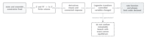
The finite-volume partition function generates response, Legendre transforms change controlled variables, and large-deviation rate functions encode phase weights only after the thermodynamic-limit order is declared. Solid connections show the primary relation; dashed outlines or arrows mark qualifications and failure boundaries. The diagram is schematic and not to scale.

The surrounding discussion supplies the relevant equations and checks in text form; the figure is a navigational summary.

Exercise

Show that the grand-canonical number susceptibility of one bosonic mode is $\partial_\mu\langle n\rangle=\beta n(1+n)$ for $\mu<\omega$.

Solution

With $n=[e^{\beta(\omega-\mu)}-1]^{-1}$, differentiation gives $\partial_\mu n=\beta e^{\beta(\omega-\mu)}/[e^{\beta(\omega-\mu)}-1]^2=\beta n(1+n)$. The divergence as $\mu\to\omega^-$ signals loss of stability of the uncondensed single-mode description.

References

• Callen, Herbert B. Thermodynamics and an Introduction to Thermostatistics. 2nd ed. New York: Wiley, 1985.
• Kardar, Mehran. Statistical Physics of Particles. Cambridge: Cambridge University Press, 2007. doi:10.1017/CBO9780511815898.
• Kubo, Ryogo. “Statistical-Mechanical Theory of Irreversible Processes. I.” Journal of the Physical Society of Japan 12, no. 6 (1957): 570–586. doi:10.1143/JPSJ.12.570.

References

Section titled “References”- Kubo, Ryogo. “Statistical-Mechanical Theory of Irreversible Processes. I. General Theory and Simple Applications to Magnetic and Conduction Problems.” Journal of the Physical Society of Japan 12, no. 6 (1957): 570–586. doi:10.1143/JPSJ.12.570; Open PDF.
Further reading
Section titled “Further reading”- Callen, Herbert B. Thermodynamics and an Introduction to Thermostatistics. 2nd ed. New York: Wiley, 1985.