

Markov-Chain Sampling of Lattice Fields
A Markov chain samples a regulated lattice field theory correctly only when its transition kernel preserves the declared target measure, communicates across every target-supported sector relevant to the observable, and is run under conditions for which a law of large numbers applies. Detailed balance is a convenient sufficient route to stationarity, not the definition of correctness; acceptance rate and short autocorrelation are efficiency diagnostics, not substitutes for invariance or coverage. This page makes those distinctions at a finite regulator, where every object can be defined and, on a small lattice, checked exactly.
Required background. Markov generators, ergodicity, and sampling error supplies transition kernels, invariant measures, and ergodic averages. Scalar actions and difference operators supplies the finite Euclidean action whose Boltzmann weight is sampled.
Helpful background. Probabilistic convergence and limit theorems supplies laws of large numbers and central-limit hypotheses.
Finite-regulator target and transition kernel
Section titled “Finite-regulator target and transition kernel”On a finite lattice, let be the configuration space and let the Euclidean action define
The reference measure is counting measure for discrete spins, Lebesgue measure for noncompact scalar variables, or the product Haar measure for compact links. The normalization need not be known to form ratios. This chapter assumes a nonnegative, normalizable weight. Complex or sign-indefinite weights require the methods and qualifications of sign problems and finite density.
Local regulator and convention card. The main benchmark is a periodic four-site Ising ring, and , with dimensionless coupling and action . General formulas use a finite or standard Borel state space, a time-homogeneous kernel , and row-vector convention . All generated-chain expectations are distinguished from exact target expectations .
A Markov kernel assigns a probability measure to the next configuration given . The target is invariant when
for every measurable set . For a finite state space this is the matrix equation . The stronger reversible, or detailed-balance, condition is
Integrating either side over proves invariance. The converse is false: a directed probability current can circulate while leaving invariant. Therefore a nonreversible kernel is not suspect merely because detailed balance fails; it must instead come with a direct stationarity proof and the same support and convergence checks.
For importance sampling from an independent proposal , the identity
requires wherever contributes and sufficient moments for the estimator used. Markov-chain sampling instead changes the distribution of the draws through ; it does not remove the support condition.
The figure below places the two Markov-chain obligations in their necessary order. Inspect the separate invariant-kernel and coverage gates: neither acceptance nor autocorrelation appears until both have passed.
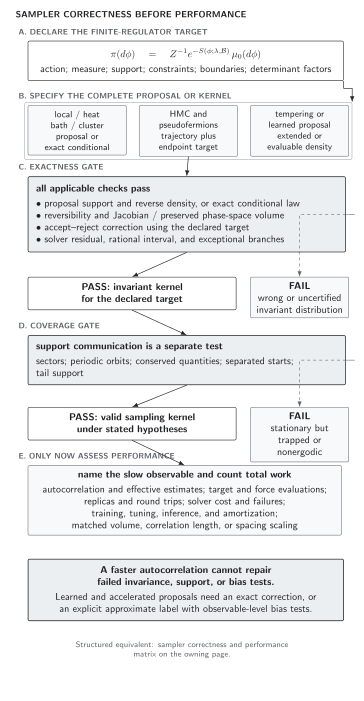
For a Markov chain, stationarity establishes the invariant distribution while support communication establishes the scope of ergodic averages. Only a kernel that passes both gates may be compared by observable autocorrelation and cost. Original schematic, not to scale.
The canonical sampler correctness and performance matrix gives the corresponding structured checks for every update family in this chapter.
From stationarity to a valid field estimator
Section titled “From stationarity to a valid field estimator”Suppose is generated by . The usual estimator is
If , then every marginal is already , so . This statement does not imply that one trajectory explores the target. If a kernel merely flips all spins, , the Ising measure is invariant and the chain is reversible, yet it remains in a two-state orbit. An ergodic theorem additionally needs the chain to communicate across the relevant support and avoid a purely periodic obstruction. On a finite state space, irreducibility plus aperiodicity is a standard sufficient pair; on general state spaces the corresponding recurrence and irreducibility conditions require a measure-theoretic formulation Tierney 1994, §§2–3.
When , the expectation at step is , not . Discarding an arbitrary number of early states does not prove the remaining bias negligible. Convergence must follow from a kernel-level argument and be challenged with starts in separated regions. After convergence, correlated draws still change the variance. For a stationary scalar observable,
where and . The limit of the bracket, when it exists, is twice the integrated autocorrelation time in the convention of Chapter 6. Estimating it from realized chains, choosing windows, and propagating it into uncertainties belong to statistical inference and error budgets. Here it appears only to separate correctness from efficiency.
Metropolis–Hastings as a stationarity construction
Section titled “Metropolis–Hastings as a stationarity construction”Let propose from . When forward and reverse proposal densities exist on the same support, accept with
The off-diagonal transition density is ; rejected proposals supply the diagonal probability. Multiplication by gives
which is symmetric under . Thus the accepted moves obey detailed balance, and the rejection term is automatically symmetric on the diagonal. This is the Metropolis–Hastings construction introduced in its general form by Hastings 1970, pp. 97–109, extending the symmetric-proposal method of Metropolis et al. 1953, pp. 1087–1092.
Two qualifications matter in field theory. First, if but , the proposed move cannot be accepted by this reversible construction. Second, a correct ratio does not establish irreducibility: the proposal may conserve a hidden parity, topological sector, or boundary value.
An exactly enumerable four-spin benchmark
Section titled “An exactly enumerable four-spin benchmark”The sixteen configurations of the periodic ring fall into three bond-energy classes. Their exact partition function is
Global spin-flip symmetry gives for . Differentiating gives the nearest-neighbor correlation
For a single-spin-flip proposal, choosing one site uniformly and setting changes the action by
so the symmetric-proposal acceptance is . Enumerate all sixteen rows of the resulting transition matrix. Each row must sum to one, every entry must be nonnegative, and the exact weights must satisfy both
These are exact algebraic checks, not noisy Monte Carlo comparisons. The single-spin proposal also connects the full hypercube and has a positive rejection probability at , establishing irreducibility and aperiodicity. Only after these generator checks should sampled estimates of be compared with the closed form above.
Adversarial failures
Section titled “Adversarial failures”A stationary but nonergodic chain. Replace the update by a global spin flip. The exact stationarity and detailed-balance residuals still vanish, but every bond product is conserved. Chains started in the ferromagnetic and alternating configurations never agree on . This negative control proves why invariance alone is insufficient.
An asymmetric proposal treated as symmetric. Bias the proposed site or direction in a state-dependent way, but accept with . The missing factor produces a nonzero balance residual and generally a wrong stationary distribution even if the acceptance rate looks healthy.
A correct kernel with a misleading short run. At large , a local chain can remain near one magnetized phase over the recorded interval. Symmetry-related starts and exact enumeration expose the finite-time failure; neither deleting a convenient prefix nor reporting repairs it.
Observable-level validation checklist
Section titled “Observable-level validation checklist”- Declare , , boundary conditions, parameter values, and the support on which is positive.
- Prove invariance—by detailed balance or a direct calculation—for the implemented transition including rejection and exceptional branches.
- Test row normalization, nonnegativity, support communication, conserved quantities, and periodicity on the smallest exactly enumerable lattice.
- Compare at least two symmetry-separated starts and one independent kernel against exact , , and another observable sensitive to sector trapping.
- Inject a missing proposal ratio or a support-preserving global flip and require the planned residual or cross-start test to fail.
- Record efficiency separately: proposal cost, acceptance, slow observable, autocorrelation convention, and cost per effective estimate. Chapter 6 determines the uncertainty from the realized chain.
Learning outcomes
Section titled “Learning outcomes”After completing this page, you should be able to:
- prove invariance of a finite-lattice transition kernel, or identify the exact correction factor that restores it; and
- distinguish stationarity, ergodicity, finite-time initialization bias, autocorrelation, and computational efficiency by tests that can fail independently.
Exercises
Section titled “Exercises”1. Prove the Ising normalization. Count the four-spin configurations by the number of domain walls and recover .
Solution
Periodic spins have an even number of domain walls. There are two configurations with zero walls, weight each; choose two of four bonds for the walls and one initial spin, giving configurations of weight one; and there are two alternating configurations with four walls, weight each. Their sum is .
2. Separate invariance from ergodicity. Write the transition matrix for the deterministic global flip on the sixteen spin configurations. Show that but exhibit a target observable whose time average depends on the starting orbit.
Solution
The matrix has and all other entries zero. Because , , so . Each orbit is only . The bond correlation is constant on such an orbit: it equals from an all-aligned start and from an alternating start, while the target value lies strictly between them at finite .
References
Section titled “References”- Hastings, W. K. (1970). “Monte Carlo sampling methods using Markov chains and their applications.” Biometrika 57(1), 97–109. doi:10.1093/biomet/57.1.97.
- Metropolis, N., Rosenbluth, A. W., Rosenbluth, M. N., Teller, A. H., and Teller, E. (1953). “Equation of state calculations by fast computing machines.” The Journal of Chemical Physics 21(6), 1087–1092. doi:10.1063/1.1699114.
- Tierney, L. (1994). “Markov chains for exploring posterior distributions.” The Annals of Statistics 22(4), 1701–1762. doi:10.1214/aos/1176325750.